This post is a continuation of Having trouble learning Lagrangian mechanics, looking at electronic systems rather than mechanical ones. Again, this is not intended as a tutorial but a dump of my understanding, to clarify it in my own head, and to get corrections or suggestions from my readers, many of whom are far better at physics than me.
For electronics, I’ll use charge  as my coordinate, with current $i = \dot q$ as its derivative with respect to time. In all but the simplest circuits, there will be multiple charges or currents involved, which I’ll distinguish with subscripts.
Some notation:
 is the difference between kinetic and potential energy of the system. The potential energy will be the energy stored in capacitors,
  , and the kinetic energy the energy in the inductors,
  . (Note: that is only self-inductance. If we have mutual inductance
  between two inductors, we need to use
  for the kinetic energy—I’m a bit confused by that, as we could have negative kinetic energy. I rarely use inductors or transformers in my electronics, so I’ve not had to work out my confusion yet.)
 is the power dissipated by the resistors in the system:
  .
. is the vector input to the system needed to make the energy balance work out. By using charge for each coordinate, the units here will be volts.
With this notation, the basic formula is
Let’s check the units:
- Potential energy:
 , which is indeed volts.
- Kinetic energy:
 , which is also volts.
- Dissipated power:
 , which is again volts (Ohm’s Law).
Now all we need to do is to figure out which  or
or  has to be associated with each component of the system, and what voltages the
  correspond to. I think that will be easiest if I have some specific circuits to work with. Let’s start with a very simple one:

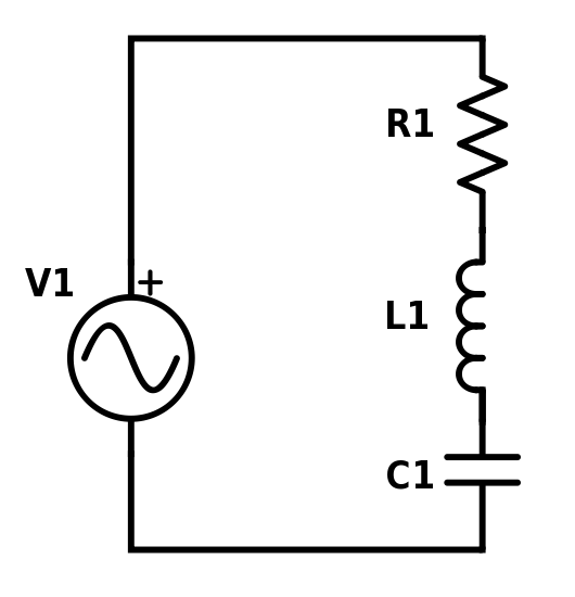
Simple RLC series circuit with a voltage source.
We can use a single coordinate, the charge on the capacitor,  , so that the current flow
  is clockwise in the schematic. We get the Lagrangian
  The power dissipation is
  , and taking the derivatives gives us
  , which is the voltage for the voltage source.
For electronics modeling, we often want to look at the ratio of two different voltages in a system, for example, the output of a filter relative to the input to a filter. How do we set that up? Let’s look at a very simple low-pass RC filter:

The upper schematic shows the normal way to represent the low-pass filter. The lower schematic shows it with a voltage source and a voltmeter, with two loops (one of which has no current).
The potential energy is just  , there is no kinetic energy (no inductors), and the dissipation is
  . Taking the derivatives of the Lagrangian gives us
 and
and
 .
.
In other words, we get the voltage at the voltage source and the voltage at the voltmeter. If we want to do anything with these equations, we need to recognize that the  and
and  terms are 0 (modeling the voltmeter as a perfect infinite impedance), giving us the usual formulas for the input and output voltage, in terms of the charge on the capacitor:
  and
and  .
.
If we take Laplace transforms, we get  and
and  , which gives us the transfer function
  , as expected. (Plug in
  to get the usual format in terms of angular frequency.)
I could do another, more complicated example, but I think that the idea is clear (to me):
- Make a charge (and current) coordinate for each current loop in the circuit—including a dummy loop with current 0 wherever you want to measure the voltage.
- Set up the Lagrangian by adding terms for each inductor (kinetic energy) and subtracting terms for each capacitor (potential energy), and set up the power-dissipation functions by adding terms for each resistor.
- Take the appropriate derivatives to get the voltages.
- If needed, eliminate charge terms by using more easily measured voltage terms.
I don’t find this process any simpler than using complex impedances and the usual Kirchhoff laws, but it isn’t much more complicated. It may be easier to use the Lagrangian formulation than setting up the equations directly when there are mutual inductances to deal with—I’ll have to think about that some more.
Of course, the big advantage I’ve been told about for Lagrangian mechanics is in electromechanical systems, where you model the mechanical part as in Having trouble learning Lagrangian mechanics and the electronic part as in this post, with only a conservative coupling network added to combine the two. It is in setting up the coupling network that I get confused when trying to model electromechanical systems, and I’ll leave that confusion for a later post.


")
 or hardback ($198)")

