OpenScope MZ review

During the CyberWeek sales I bought myself an OpenScope MZ USB scope from Digilent, to see how it compared with the Analog Discovery 2, which I use frequently.  I particularly wanted to see whether I could recommend it as a low-cost alternative ($89 list) for the AD2 ($279 list, but $179 with academic discount).

I’ve not had a chance to do much testing yet, but the short answer is that I would recommend saving up for the Analog Discovery 2—the OpenScope MZ is nowhere near being a professional instrument, but the AD2 is close.

The first thing I tested was the function generator.  The OpenScope MZ does not have a real DAC, but uses digital output pins and a resistor ladder to generate analog voltages.  The result is a “DAC” that is non-monotonic.  The non-monotonicity can be observed by generating a sawtooth waveform and observing the result with an Analog Discovery 2.

The non-monotonicity is worst when the DAC switches from 0x1ff to 0x200 (from 511 to 512 out of 1024 steps). This was a 3Vpp sawtooth at 10Hz. The OpenScope MZ also has a much larger offset than the AD2.

To get clean measurements, I set the AD2 to average 100 traces.  I also did 16-fold oversampling, so that I could get good time resolution while recording the whole period.

The steps are not of uniform duration, but don’t seem to be a simple pattern of single or double clock pulses:

The step durations vary here from 64µs to 136µs in this small sample, but with 1024 steps in 0.1s, I would expect 97.66µs.

The step heights are not completely consistent either, but seem to average to roughly the right value:

The step size should be 3V/1024=2.93mV, but in this range the average step size is a little high. (but the first step at the bottom left is too small).  The variable duration of the steps is also very visible here.

The speed limitations of the amplifier for the OpenScope’s function generator are also quite clear:

There seems to be a 12V/µs slew rate limitation, and the large step at the end of the sawtooth has a 258ns fall time. By way of contrast, the AD2 has about a 40ns fall time for the same 10Hz ramp up and a slew rate of about 120V/µs.

I found the Analog Discovery 2 falling edge rather interesting—the stepwise descent may be an artifact of recording the waveform with the same instrument used for generating it (so that the oversampling does not work correctly), but it might also indicate that the ramp edge is digitally pre-filtered to keep it from overshooting.

Santa Cruz Mini Maker Faire 2017

Today I spent about 10 hours on the 2017 Santa Cruz Mini Maker Faire.  The hours for the Faire were 10–5, but I spent some time setting up and tearing down afterwards, so I left the house around 8:30 a.m. and had the bike trailer unpacked and everything back in the house by about 6:30 p.m.  I figure that I spent only about 10 hours earlier on setup for this Faire: applying for the Faire, setting out all the displays and testing them at home, preparing new blurbs for my book and blog, making table signs telling people how to use the interactive parts of the display, blogging about the Faire, and doing load-in last night.  That is a lot less than last year, as I was able to reuse a lot of the design from last year.

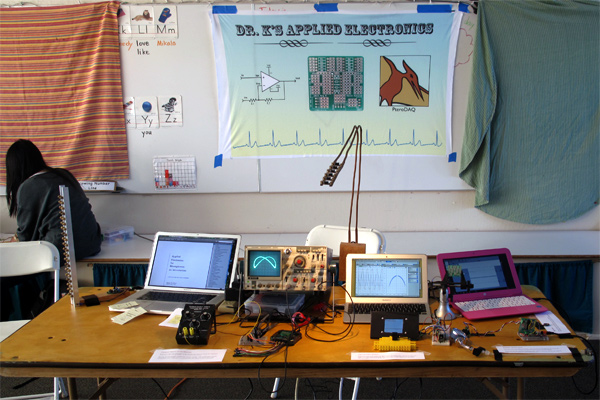
Here is the table display I ended up with:

The bare corner at the front left was reserved for the students in my freshman design course who were coming to display their muscle-controlled robot arm, but they decided to set up in back (you can see one of the lead students in the background).

I had four interactive displays (from left to right):

• A pair of function generators and an oscilloscope showing Lissajous figures.  I changed this from last year, as I did not use the FG085 function generator this year, but one of the function generators from the Analog Discovery 2.  I still used the Elenco FG500, despite the very low quality of its waveforms, because it has a knob that is easy for kids to turn, and is easy to reset if they mess it up (unlike the jamming buttons on the FG085).  I did not use the second function generator on the Analog Discovery 2, as I did not want kids playing with just a software interface (and a rather complicated one at that).  It might even be worthwhile for me to build a simple audio sine-wave oscillator with a single big knob over the summer, so that I can have something for kids to play with that is fairly robust and that can’t be easily set into a weird state.  I could even do two, just for Lissajous figures, though having one fixed oscillator worked well this time.  I had the Analog Discovery 2 oscilloscope showing on the laptop next to the old Kikusui CRT oscilloscope, showing both the waveforms and the XY plot, so that I could explain to adults what was happening with the Lissajous figures and about the differences between classic oscilloscopes and modern USB-based ones.
  A lot of people asked me about the Analog Discovery 2, which I was very enthusiastic about—Digilent should be giving me a commission! (They aren’t, although I’m sure I’m responsible for at least half a dozen sales for them, and a lot more if we go ahead with our plan to use them in place of bench equipment in my class next year.)
• In front of the laptop showing the Lissajous figures, I had a standalone optical pulse monitor using the log-transimpedance amplifier and the TFT LCD display.  Using the log-transimpedance amplifier worked well, as did using a lego brick to block light to the sides and back of the phototransistor.  A lot of people have trouble holding their hands still enough to get good readings (particularly children), so it would be good to have some sort of clip instead of resting a finger over the phototransistor.  I’ve tried making clips in the past, but I’m not good at mechanical design, and I’ve always ended up with either a clamp that is too tight (cutting off circulation and getting no reading) or too loose (falling off).  Ideally, I’d want a pressure between systolic and diastolic pressure, so about 12kPa (90mmHg).  People did like the use of Lego as a support, though—it provided a familiar element in the strange world of electronics.
• To the right of the pulse monitor was a pressure sensor.  I had a mechanical gauge and the electronic sensor both connected to a piece of soft silicone tubing taped to the table top.  Kids pressed on the tubing to get an increase in pressure, visible on the gauge (about 20–60 mmHg) and on graph PteroDAQ was running on the little laptop (which we refer to as the “Barbie” laptop, because of its color and small size).  I explained to kids that the tubing was like the tubing stretched across roads sometimes to count cars, with a pressure sensor that recorded each pulse as wheels compressed the tubing.  (For some of the old-timers, I reminded them of when gas stations used to use a similar system.)
  PteroDAQ worked well for this setup, running all day at 20 samples per second without a glitch.  The only problem was occasional display sleep from the laptop, fixable by touching the touch pad.
• At the far right end of the table, I had a phototransistor which kids could shadow with their hands, with the result visible on another channel on PteroDAQ.  This was a last-minute change, as I was getting very unreliable results from the capacitive touch sensor when I tested it out last night.  The capacitive touch sensor worked fine at my house, but in the kindergarten room at Gateway I has a different electrical environment, and it would not work unless I grounded myself. Rather than fuss with the touch sensor, I made a new table sign and put in a light sensor instead.
  I might want to experiment this summer with different ways of making touch plates—trying to get one that doesn’t rely on the toucher being grounded.  My initial thought is that if I have two conductors that are not too close together, but which would both be close to a finger if the touch plate is touched, then I may be able to get more reliable sensing.  I could try some wire-and-tape prototypes and maybe make PC boards with different conductor layouts.  (OSH Park‘s pricing scheme would be good for such tiny boards).

I also had my laptop displaying my book; some quarter-page blurbs with URLs for my book, PteroDAQ, and this blog; my 20-LED strobe; my desk lamp; and a PanaVise displaying one of the amplifier prototyping boards.

I’d like to think of a more exciting project for kids to play with next year—perhaps something I could build over the summer.  Readers, any suggestions?

In addition to my display, some of the freshmen from my freshman design seminar class demonstrated their EMG-controlled robot arm (which uses the MeArm kit):

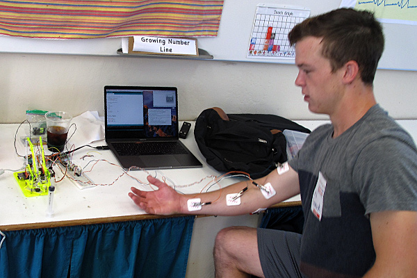
The students built a MeArm from a kit, then programmed a Teensy board to respond to muscle signals amplified by amplifiers designed by other students in the class. The combined project had two channels: one for controlling the forward-backward position of the arm (using the biceps), the other for controlling the gripper (using muscles in the forearm). With practice, people could pick up a light object with the robot arm.

The scheduling of the Mini Maker Faire was not ideal this year, as it conflicted with the Tech Challenge, Santa Cruz County Math contest, the California Invention Convention, and the Gem and Mineral Show, all of which draw from the same audience as the Mini Maker Faire.

The Faire seemed to be reasonably well attended (rather slow for the first hour and half, but picking up considerably in the afternoon).  There was plenty of room for more exhibitors, so I think that organizers need to do a bit more outreach to encourage people to apply.  It would probably help if they were quicker responding to applicants (it took them over three months to respond to my application, and then only after I nudged them).

Some obvious holes in the lineup: The Museum of Art and History did not have a display, but I saw Nina Simons there, and she said that MAH definitely plans to do it next year, but the Abbott Square renovation is taking up all their time this year.   The fashionTEENS fashion show was April 21, just over a week ago, so it would have been good to get some of them to show their fashions again: either on mannequins or as a mini-show on the stage.  It might be good to get some of Santa Cruz’s luthiers or fine woodworkers to show—we have a lot of top-notch ones, and many do show stuff at Open Studios. The only displays from UCSC were mine and the Formula Slug electric race car team.

Of the local fab labs, Cabrillo College Fab Lab and Idea Fab Labs were present, but The Fábrica and the Bike Church were not.  I thought that Cabrillo did a great job of exhibiting, but Idea Fab Labs was a little too static—only the sand table was interactive.

It might be good to have Zun Zun present their Basura Batucada show (entirely on instruments made from recycled materials) and have a booth on making such instruments.  It might be hard to get Zun Zun to volunteer, but they used to be very cheap to hire (I hired them to give a show at my son’s kindergarten class 15 years ago—they were very cheap then, but I don’t know what their prices are now).

One problem my wife noted was the lack of signs on the outside of classrooms, so that people would know what was inside.  The tiny signs that the Faire provided (I think—I didn’t get one) were too small to be of any use.  It may be enough to tell makers to bring a poster-sized sign to mount.  I had my cloth banner behind my table, but a lot of the displays were hard to identify.  Instructions or information mounted on tables would also have been good—again these would have to be provided by the makers.  I did not see people carrying maps this year—they can also be helpful in getting people to find things that were tucked away in odd corners.  Not many people made it back to the second kindergarten room where FabMo and the Lace Museum activities were.

Update 2017 May 1: It turns out that there were some things I missed at the Faire.  The principal of Gateway sent me email:

… we did have 4 of the Fashion Teens exhibit their creations on the stage at 11:30—might be cool to have them put those on mannequins and have a booth next year. Also we had two more UCSC projects—Jim Whitehead and the Generative Art Studio, and Project AWEsome from the School of Engineering. We would LOVE to have more UCSC-related projects …

 

FET I-vs-V with Analog Discovery 2 again

 

In FET I-vs-V with Analog Discovery 2, I plotted Id vs. Vgs curves for an nFET:

The Ids-vs-Vgs curves do not superimpose as nicely as curves I’ve measured with PteroDAQ. I don’t yet understand why not.

Yesterday, I played with sweeping the power supply (Power waveform generator).  In this post, I used that capability to plot Id vs Vds curves for different gate voltages (Vgs) of a different nFET (since the AOI518 is an obsolete part).  The setup is the same as for the previous test—the function generator is connected to the gate, the power supply to the drain load resistor in series with the nFET whose source is connected to ground, and the two oscilloscope channels monitor the voltage across the load resistor and across the nFET.  The difference is that I use the power-waveform option to put a 1Hz triangle wave on the power supply, but put just a DC offset (AC amplitude 0V) on the function generator output, so that the gate voltage is constant as the drain voltage is adjusted.

The saturation regions are well plotted up to Vgs=2.7V. I averaged 10 or 20 scans for each of these curves, to reduce quantization noise for small voltages or small currents.

I got quite different results when I removed and replaced the nFET from the breadboard—the breadboard contacts seem to have a variation of about ±0.05Ω in resistance, which is much larger than the on-resistance of the nFET when fully on. I took measurements with a wire between the source and drain to estimate the wiring resistance, but wiggling the wire produced very different results.

In the next graph, I tried subtracting off the wiring resistance to get the on-resistance, but I’m really quite dubious about the measurements smaller than 0.5Ω, because of the unrepeatability of the bread board contact resistance.

The numbers here look good (close to the spec sheet), but repeating the measurements could result in ±0.1Ω, which makes the Ron measurements for fully on transistors rather useless.

By using a smaller power resistor, I could probably get saturation currents for slightly higher gate voltages, up to the current limit of the power supplies in the Analog Discovery 2, but better on-resistance measurements would require a better jig for making low-resistance contacts to the FET.

By using a much larger resistor, I could measure low currents more accurately, which would give me a better idea of the leakage currents—I don’t really believe the measurements for Vgs=2.1V, because the current appears to decrease with increasing Vds, which is probably an artifact of measuring a small difference in voltage with a large common-mode signal.

I tried using larger resistors to measure the saturation currents, but the results varied a lot depending on what size load resistor is used. I believe that the difference is due to temperature changes from self-heating. If I sweep out to larger Vds voltages (using a smaller load resistor, hence smaller IR drop across it), but about the same saturation current, I’m dissipating more power in the transistor, so making it warmer. This appears to increase the saturation current. Reducing the range of the voltage with the same load resistor drops the curve down, just as increasing the load resistor does. I suspect that proper measurement requires a jig that holds the transistor at a nearly constant temperature, as well has having very low contact resistance.

The saturation current seems to vary by about ±10% as I change load resistors. The effect is most likely thermal—note that using a smaller voltage sweep for Vgs=2.3V and Rload=51Ω resulted in almost the same curve as Rload=270Ω, because the power dissipated was about the same.

Note that the thermal explanation also works for explaining why the superposition does not work well for the Id vs Vgs plots—at lower load resistances, more power is dissipated in the transistor, and it gets warmer, shifting the current curve upward.

Power waveform generator

I was playing around a little more today with my Analog Discovery 2 USB oscilloscope, and found that one could set up the power supplies to be high-power waveform generators by setting configuration 6 in the device manager.  The power supplies are not great function generators, of course, as they are switching power supplies, but I can see some use cases for this functionality.

The power supplies are nominally limited to 700mA, so I wondered whether they had the same sort of sharp clipping that the function generator has (see FET I-vs-V with Analog Discovery 2).  I tested the power waveform generator with several different loads:

With no load, the power supply waveform generator has trouble with small voltages (no resistance to drain the capacitance) and has fairly high noise, but is nicely linear. At high load (1.8Ω) the voltage is substantially less than specified.

We can get a clearer idea of the behavior by looking at the difference between the power waveform generator and the normal waveform generator:

At low voltages, the regulator’s output capacitor is not discharged fast enough without a load resistor. The regulator also does a better job of keeping the noise down with higher load.

With no load, the noise on the power waveforms is about ±4mV, but at high load, it drops to about ±1mV.

The noise is periodic with a frequency of about 1.024kHz, which is much too low a frequency for a switching regulator—it is actually from the sampling frequency for the waveform generator generating a 1Hz triangle wave (2¹⁰ samples in wavetable). The usual waveform generator has four times as high a sampling frequency, so the error is mostly just quantization error from the power waveform generator, though a single step from the power waveform generator takes about 250µs to settle, so the 1Hz maximum frequency for the power waveform channels seems reasonable. With a 10Ω load, the settling time is reduced to about 50µs and the noise on each step is about 500µV RMS (not counting the quantization error).

With the 1.8Ω load, I let the current get as high as 927mA (well above the 700mA specification), and there is no sign of clipping. We can more reasonably model the power waveform generator as having an internal resistance. For the 1.8Ω and 10Ω loads, I plotted the equivalent internal resistance as a function of voltage (for the larger voltages):

The internal resistance is approximately 100mΩ—180mΩ, with the larger values at higher voltages. There is a clear anomaly at half the full-scale voltage (2.5V for 10Ω and 0.9V for 1.8Ω).

I believe that the power waveforms will be useful for characterizing transistors, especially for sweeping a range of V_ds voltages that require a substantial current.

Function generator bandwidth of Analog Discovery 2

The network analyzer function of the Analog Discovery 2 USB oscilloscope makes it easy to characterize the function generator’s bandwidth—just connect the function generator to the input channel (making sure that the input channel is not specified as a reference) and do a sweep.  The only choice is whether to use the wires that come with the basic unit or the optional BNC adapter board and scope probes.  I tried it both ways (and with both 1X and 10X settings of the scope probes), using 1V amplitude on the waveform generator one in all cases:

There is not much difference in the bandwidth between 10X probes and wires (both high impedance) (8.5–8.8MHz bandwidth), but the 1X scope probes provide higher bandwidth—higher than the 10MHz measurable with the network analyzer.

I tried loading the function generator with resistors, but this made essentially no difference in the frequency characteristics. It isn’t the 1MΩ resistance of the scope that matters, but the capacitance of the oscilloscope plus probe.

So I tried adding capacitive loads and found that I got a very clear LC resonance. With a 330pF load, I got the peak near 10MHz to approximately cancel the drop:

The resonance around 9.1MHz with a 330pF load is actually a little too strong and over-corrects for the drop in bandwidth. Adding 6.8Ω in series with the 330pF capacitor makes a load that nicely compensates for the inductance of the wires.

A resonance around 9.1MHz with a 330pF capacitor implies an inductance of about 0.93µH, which is in a reasonable ballpark of the sort of inductance one would expect for 80cm of wire (4 wires each about 20cm).