Changing the loudspeaker lab

I’ve started looking at how the loudspeaker lab in the applied-electronics course will change, given that we will have the Analog Discovery 2 USB oscilloscope in the labs.  There are two main changes in capabilities:

• hundreds of measurements can be made in a couple of minutes from 10Hz to 1MHz
• phase information is available, not just amplitude information.

The availability of phase information means that we can try fitting complex impedance, and not just the magnitude of impedance.  Unfortunately, the gnuplot curve fitting that we’ve been using is only set up for fitting real-valued functions, not complex-valued ones, and I don’t really want to switch to a more full-featured model fitting program, as they get hard to use.

Today I gathered data from two loudspeakers: the tiny 1cm one that I have posted about before (Ultrasonic rangefinder tests with tiny loudspeaker and Redoing impedance test for tiny loudspeaker) and an 8Ω oval loudspeaker that we used to use in the class until Parts Express sold out of them (Loudspeaker analysis, Better model for loudspeaker). I only collected data out to 1MHz, since my previous experience indicated that the network analyzer was not very useful past that frequency (Loudspeaker impedance with Analog Discovery 2). I put a 22Ω resistor in series with the loudspeaker and measured the voltage across it on channel 1, with the voltage across the loudspeaker on channel 2.  I recorded the “gain”, which is channel2/channel1, and the phase for channel 2 relative to channel 1.  The gain times 22Ω is the magnitude of the impedance of the loudspeaker.

The formula that I’ve been using for impedance modeling, , turned out not to be a good fit for the phase.  I played around for a couple of hours with different, more complicated models, before finally settling on a model that is as simple as the one I’ve been using, but that fits pretty well:

The difference is just that I’m including the j inside the exponentiation, so that the “inductor-like” component is now in direction instead of —that is, the asymptotic phase angle is instead of 90°.

To do the fitting, I alternated between fitting some of the parameters to the magnitude of the impedance and some to the phase. After I had layed around a bit and gotten ball-park estimates of the parameters, I did a more careful fitting. I started by fitting the series R to just the low-frequency end of the data, then fitting the resonance peak without the “inductor-like” component in the model with data collected in just a decade of frequency around the resonance peak (I used a separate data file that had 600 data points for just that decade).  I fit the three parallel parameters using the phase data, then refit the parallel resistance using the amplitude data.  To start in the right region, I set initial values , , and , with being the magnitude of the impedance at the top of the peak, located at frequency , with .

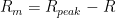
With those parameters set, I fit with phase information for the high frequencies, and with amplitude information.

I then tweaked the fit by refitting the resonance peak, refitting and , and repeating the refits.

The 6-parameter fit for the magnitude is pretty good.

The 6-parameter fit for the oval loudspeaker is not great for phase, but is not too bad.

The 6-parameter fit for the tiny loudspeaker is pretty good, though I did not attempt to model the two higher frequency resonances that are visible, despite knowing that the resonance around 9kHz rings seriously.

The resonances are somewhat more visible in the phase plot for the tiny loudspeaker than they are in the magnitude plot.

I’m going to have to write up a tutorial for the book on using a real-valued fitting method for fitting a complex-valued function.

Fidget spinners revisited

In Fidget spinners, I wrote about measuring and modeling the acceleration of two fidget spinners, 5-spoke spinner that cost $6.90 made from plastic and brass and a 3-bladed spinner that cost $8.90 milled out of brass:

The 5-spoked wheel spinner weighs 32.88±0.03g, and the 3-spoke brass spinner weighs 61.14±0.02g.

The previous post looked only at the fidget spinners spinning vertically (that is, with a horizontal axis), but I had noticed in playing with the spinners that they seemed to have different drag in different orientations, so I redid the measurements with the spinners horizontal (that is, with a vertical axis). I had a somewhat harder time spinning the spinners fast with them horizontally mounted, as my makeshift support for the photointerrupter was a bit precarious.

The 5-spoke wheel seemed to run smoothly , but the fit suggests more dry friction and less fluid friction.

The 3-spoke spinner really does not like to spin horizontally.

To visualize the physics better, I tried making acceleration vs. velocity plots for the fitted models:

When holding the wheel horizontally, there seems to be mainly dry friction, almost independent of the speed of the spin.

The 3-spoke spinner has much worse drag at all speeds when held horizontally rather than vertically. The fluid drag seems to be about the same as before, but there is much larger dry friction component (possibly from brass-on-brass contact between the spinner and the axle caps).

As expected from fidgeting with the spinners, the 3-blade spinner has much more drag than the wheel, both horizontally and vertically. The change from mainly wet friction to mainly dry friction for the wheel was unexpected, though.

Update 2017 Jun 25 21:15:  My wife just pointed me to a Wired article: https://www.wired.com/2017/05/the-phyiscs-of-fidget-spinners/ which does a poorer job of the same thing I did. They sampled at a fixed rate, rather than recording time stamps on each rising edge, so they had much poorer time resolution, and they assumed constant acceleration (dry friction), which is only appropriate for low-quality bearings.

Uncompensated transimpedance amplifier

In my book Applied Electronics for Bioengineers, I have students build transimpedance amplifiers for phototransistors (and some students use them for electret microphones as well).  In the book, I never deal with compensating the transimpedance amplifiers to avoid oscillation, as I try to stay away from students having to reason about phase of signals and oscillation has never been a problem in the student designs.

But I thought that I ought to understand the method myself, especially if I need to help students trying to do higher bandwidth, higher gain transimpedance amplifiers.  First I read up on the subject—one of the better introductions is the Maxim application note 5129 Stabilize your transimpedance amplifier.  The key concepts are the following:

• When the frequency is high enough (where the open-loop gain is limited by the gain-bandwidth product) the phase change of the amplifier is about –90° (or 90° for the negative input).
• If we set up a transimpedance amplifier with feedback resistor R, then the feedback consists of a low-pass RC filter: a voltage divider with R on tap and the input capacitance of the amplifier and any capacitance in parallel with the current source on the bottom.
• The phase change of a low-pass RC filter (gain ) approaches –90° above the corner frequency.
• Having a phase change of 0° and gain ≥ 1 around a feedback loop results in instability and possible oscillation.

That means that we can have instability at frequencies between and the gain-bandwidth product (though we probably only have problems for frequencies at least a factor of 3 above the low-pass corner frequency, since the phase change of the filter is only asymptotically –90°).  If the parasitic capacitances are low and we only request small transimpedance gain, then RC is small, and the corner frequency of the low-pass filter is above the gain-bandwidth product, so there are no problems.  Will the students ever encounter problems?

Today I tried to make an unstable transimpedance amplifier using the MCP6004 op amps that we use in class.  The op amps have a gain-bandwidth product of 1MHz, so I needed an RC time constant much larger than 160ns.  I chose 2MΩ and 47nF for an RC time constant of 94 ms and a corner frequency of 1.69Hz.

The very large bypass capacitors are to make sure that there are no sneak paths through the power supply and positive input—to make sure that I’m looking at the phenomenon I’m really interested in.

I connected the amplifier up to the Analog Discovery 2, and I definitely got instability:

There does seem to be a somewhat unstable oscillation happening.

The reasoning about the amplifier instability suggests that the oscillation should be at about the frequency where the gain around the loop is 1, that is where or . For the circuit I made, that would be around .

I did some FFTs of the waveform (averaging over hundreds of traces to reduce noise, since the signal is fluctuating).

The peak is around 1380Hz, very close to the predicted oscillation frequency. Also visible are harmonics of 60Hz, which are the correct output of the transimpedance amplifier (picking up stray currents by capacitive coupling).

To compensate a transimpedance amplifier, we need to add a small capacitor in parallel with the feedback resistor, making the gain of the feedback filter , where and are the feedback components and is the input capacitance. For “optimal” compensation, we want to set the upper corner frequency at the geometric mean of the lower corner frequency and the gain-bandwidth product . Using a larger capacitor (overcompensating) increases the phase margin (thus allowing for some variation from specs) at the cost of reducing the bandwidth of the final amplifier.

We can set the equation up as , which we can simplify by assuming that to get , which for my design comes to 61pF.

A 68pF compensation capacitor cuts out the oscillation peak, but there is still a fair amount of noise around the corner frequency of the amplifier (1.2kHz). Overcompensating with a 680pF capacitor reduces the noise substantially, but the bandwidth is reduced to 120Hz.

I also tried a somewhat more realistic example, with only a 2.2nF input capacitance, which calls for about a 13pF compensation capacitor. A 20pF capacitor does fine:

The oscillation is well suppressed by the compensation capacitor.

Now I have to decide how much (if any) of this to include in my book. Perhaps it can be an optional “advanced” section in the transimpedance amplifier chapter?

Fidget spinners

I recently bought two fidget spinners from Elecrow:

The 5-spoked wheel spinner weighs 32.88±0.03g, and the 3-spoke brass spinner weighs 61.14±0.02g.

The heavier 3-bladed spinner cost $8.90 and is milled out of brass (though the site claims “pure copper”, the material looks like brass and is slightly magnetic, so I’m sure it is brass).The lighter 5-spoke spinner cost $6.90.

The lighter spinner is easier to get to high speed, spins longer, has more gyroscopic effect, and has a dimple for balancing it on a pencil point, so makes the better fidget spinner in many ways.

I was curious whether I could characterize the fidget spinners electronically. I have a photointerrupter (an aligned LED and photodetector) from Sparkfun with a 1cm gap that the spinners just fit in.

Here is the 3-spoke spinner mounted in the Panavise Jr, with the photointerrupter counting 6 ticks per revolution.

Here is the 5-spoke spinner with the photointerrupter counting 5 ticks per revolution.

I set up PteroDAQ to record a timestamp on every rising edge of the photodetector, which counts 5 uniformly spaced ticks per revolution for the 5-spoke wheel, but 6 ticks (in 3 pair of closely spaced ones) for the 3-bladed spinner. I can then plot the angular position of the spinner as a function of time in gnuplot:

plot '3-spoke-spin-down-ticks.txt' u 1:($0/6.)

I tried fitting the spin-down using constant deceleration (a quadratic), using deceleration proportional to velocity (exponential decay), and using a model that has both terms: .  I expressed position as number of turns (that being simpler to interpret than radians), and so the initial velocity  is in turns/sec, acceleration is in turns per second per second, and the decay time is in seconds.  I got terrible fits with the constant deceleration, decent fits until the spinning got slow with the exponential decay, and quite a good fit with the combined model:

The longer spin time for the wheel is partly due to higher initial velocity, but the time constant for the decay is also much longer for the wheel, indicating better bearings.

I’m not quite sure how to interpret the slightly higher contact friction term for the 5-spoke wheel.

Kind thoughts from a student

One of my students sent me a nice e-mail at the end of the quarter.  With her permission I’m reprinting it here:

Dear Prof. Karplus,
I just wanted to take a moment to thank you and tell you how much I enjoyed the class over the last two quarters. Even though my scores may not reflect it, I feel like I’ve gotten the opportunity to learn a lot. In addition to that, some of the projects gave me a chance to spend time and connect with my father, who’s also an engineer. He was amazed at my ability to draw and build a circuit on my own (as I did the class-D lab solo), because he claims he was never able to do so when he first started learning electronics. The last project was especially very meaningful, since EKGs are  personal to me due to some childhood problems, and I got to learn how they work. I created my graduation cap as a tribute to that project and the class (see attached picture), I hope you like it!

Hope to see you at graduation,
Manisha

Manisha Marisetty’s graduation cap

A number of students in the class have told me how much they learned in the class, and not just about electronics. Other things students have mentioned include writing improvement, breaking things into subproblems, and debugging. This feedback from the students is valuable, as it keeps me motivated to keep improving the course. The course is a lot of work (for me and for the students), and it would be very easy to burn out if the course were not having much positive effect on the students.

Note: constructive criticism from the students is also useful—I’ve had several tell me that there need to be more drill exercises, for example, and there have been requests for more worked examples.  But small amounts of positive feedback help keep me motivated to do the work of addressing the problems. (Students have also suggested that I need to give more positive feedback—something I’m working on, but finding difficult to do consistently.)

I’m afraid I won’t go to the graduation ceremonies this year—I’ve got too much grading still to do, and I figure I’ll barely be completing the grading by the Tuesday deadline as it is. I’ve gotten the electrode-lab redone reports graded, and one third of the EKG labs done. I have the remaining 23 EKG lab reports to grade, an independent study, and a senior thesis. I’m on schedule, but not with a lot of time to spare.