I spent a little time today working on my book, but I got side tracked into a different project for the day: designing a super-cheap coin-cell battery connector. I’ve used coin-cell battery holders before, like on the blinky EKG board, where I used a BH800S for 2 20mm CR2032 lithium cells. That battery holder is fairly large and costs over $1—even in 1000s it costs 70¢ a piece. So I was trying to come up with a way to make a dirt cheap coin-cell holder.
The inspiration came from the little LED lights that “glovers” use inside their gloves. They are powered by two CR1620 batteries (that means a 16mm diameter and 2.0mm thickness for the battery). Because the lights have to be made very cheaply, they don’t use an expensive holder, but put the negative side of the batteries directly against a large copper pad on the PC board. The batteries are held in place by the positive contact, which is a piece of springy metal pressing the battery against the board—and each manufacturer seems to have a slightly different variant on how the clip is made.
Unfortunately, I was unable to find any suppliers who sold the little clips—though I found several companies that make battery contacts, it seems that most are custom orders.
My first thought was to bend a little clip out of some stainless steel wire I have sitting around (not the 1/8″ welding rod, but 18-gauge 1.02362mm wire). That’s about the same thickness as a paperclip (which is made out of either 18-gauge or 19-gauge wire), but the stainless steel is stiffer and less fatigue-prone than paperclips. I was a little worried about whether stainless steel was solderable, so I looked it up on Wikipedia, which has an article of solderability. Sure enough, stainless steel is very hard to solder (the chromium oxides have to be removed, and that takes some really nasty fluxes that you don’t want near your electronics). So scratch that idea.
I spent some time looking around the web at what materials do get used for battery contacts—it seems there are three main ones: music wire, phosphor bronze, and beryllium copper, roughly in order of price. Music wire is steel wire, which gets nickel plated for making electrical connections. It is cheap, stiff, and easily formed, but its conductivity is not so great, though the nickel plating helps with that. The nickel oxides that form require a sliding contact to scrape off to make good electrical connection. Phosphor bronze is a better conductor, but may need plating to avoid galvanic corrosion with the nickel-plated battery surfaces. Most of the contacts I saw on the glover lights seemed to have been stamped out of phosphor bronze. Beryllium copper is a premium material (used in military and medical devices), as it has a really good ratio of yield strength to Young’s modulus, so it can be cycled many times without failing, but also has good conductivity.
Since I don’t have metal stamping machinery in my house, but I do have pliers and vise-grips, I decided to see if I could design a clip out of wire. It is possible to order small quantities of nickel-plated music wire on the web. For example, pianoparts.com sells several different sizes, from 0.1524mm diameter to 0.6604mm diameter. I may even be able to get some locally at a music store.
My first design was entirely seat-of-the-pants guessing:
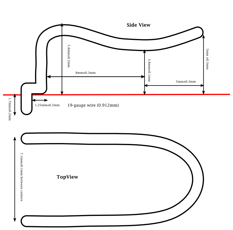
First clip design, using 19-gauge wire, with two 1mm holes in PC board to accept the wire. This design is intended for two CR1620 batteries.
The idea was to have a large sliding contact that made it fairly easy to slide the batteries in, but then held them snugly. Having a rounded contact on the clip avoids scratching the batteries but can (I hope) provide a fair amount of normal force to hold the batteries in place. But how much force is needed?
I had a very hard time finding specifications on how hard batteries should be held by their contacts. Eventually I found a data sheet for a coin battery holder that specified “Spring pressure: 50g min. initial contact force at positive and negative terminals”. Aside from referring to force as pressure and then using units of mass, this data sheet gave me a clear indication that I wanted at least 0.5N of force on my contacts.
I found another battery holder manufacturer that gave a tiny graph in one of their advertising blurbs that showed a range of 100g–250g (again using units of mass). This suggests 1N-2.5N of contact force.
Another way of getting at the force needed is to look at how much friction is needed to hold the batteries in place and what the coefficient of friction is for nickel-on-nickel sliding. The most violently I would shake something is how fast I can shake my fingertips with a loose wrist—about 4Hz with an peak-to-peak amplitude of 22cm, which would be a peak acceleration of about 70 m/s^2. Two CR1620 cells weigh about 2.5±0.1g (based on different estimates from the web), so the force they need to resist is only about 0.2N. Nickel-on-nickel friction can have a coefficient as low as 0.53 (from the Engineering Toolbox), so I’d want a normal force of at least 0.4N. That’s in the same ballpark as the information I got from the battery holder specs.
So how stiff does the wire have to be? I specified a 0.2mm deflection, so I’d need at least 2N/mm as the spring constant for the contact, and I might want as high as 10N/mm for a really firm hold on the batteries.
So how should I compute the stiffness of the contact? I’ve never done mechanical engineering, and never had a statics class, but I can Google formulas like any one else—I found a formula for the bending of a cantilever loaded at the end:
 , where F is force, d is deflection, E is Young’s modulus, I is “area moment of inertia”, and L is the length of the beam. More Googling got me the area moment of inertia of a circular beam of radius r as
  . So if I use the 0.912mm wire with an 8mm beam I have
F/d = 200E-6 mm E.
More Googling got me some typical values of Young’s modulus:
| material |
E [MPa = N/(mm)^2] |
| phosphor bronze |
120E3 |
| beryllium copper |
135E3 |
| music wire |
207E3 |
If I used 19-gauge phosphor bronze, I’d have about 24N/mm, which is way more than my highest desired value of 10N/mm. Working backwards from 2–10N/mm what wire gauge would I need? I get a diameter of 0.403mm to 0.603mm, which would be #6 (0.4064mm), #7 (0.4572mm), #8 (0.5080mm), #9 (0.5588mm), or #10 (0.6096mm), on the pianoparts.com site. I noticed that battery contact maker in Georgia claims to stock 0.5mm and 0.6mm music wire for making battery contacts, though they first give the sizes as 0.020″ and 0.024″, so I think that these are actually 0.5080mm and 0.6096mm (#8 and #10) music wire.
It seems that using #8 (0.020″, 0.5080mm) nickel-plated music wire would be an appropriate material for making the contacts. Note that the loop design actually results in two cantilevers, each with a stiffness of about 4N/mm, resulting in a retention force of about 1.6N. The design could be tweaked to get different contact forces, by changing how much deflection is needed to accommodate the batteries.
How much tweaking might be needed? I found the official specs for battery sizes (with tolerances) in IEC standard 60086 part 2: The thickness for a 1620 is 1.8mm–2mm, the diameter is 15.7mm–16mm, and the negative contact must be at least 5mm in diameter. The standard also calls for them to take an average of 675 hours to discharge down to 2v through a 30kΩ resistor (that’s about 56mAH, if the voltage drops linearly, 67mAH if the voltage drops suddenly at the end of the discharge time). If the batteries can legally be as thin as 1.8mm, then to get a displacement of 0.2mm, I’d need the zero-point for the contacts to be only 3.4mm from the PC board, not 3.8mm, and full thickness batteries would provide a displacement of 0.6mm, and a retention force of about 4.8N.
If I were to do a clip for a single CR2032 battery, I’d need to have a zero-point 2.8mm from the board, to provide 0.2mm of displacement for the minimum 3.0mm battery thickness.
So now all I need to do is get some music wire and see if I can bend it by hand precisely enough to make prototype clips. I’d probably change the spacing between the holes to be 0.3″ (7.62mm), so that I could test the clip on one of my existing PC boards.
Update 2014 July 6: I need to put an insulator on the verticals (heat shrink tubing?), or the top battery will be shorted out, since the side of the lower battery is exposed.
 as my coordinate, with current $i = \dot q$ as its derivative with respect to time. In all but the simplest circuits, there will be multiple charges or currents involved, which I’ll distinguish with subscripts.
 is the difference between kinetic and potential energy of the system. The potential energy will be the energy stored in capacitors,
  , and the kinetic energy the energy in the inductors,
  . (Note: that is only self-inductance. If we have mutual inductance
  between two inductors, we need to use
  for the kinetic energy—I’m a bit confused by that, as we could have negative kinetic energy. I rarely use inductors or transformers in my electronics, so I’ve not had to work out my confusion yet.)
 is the power dissipated by the resistors in the system:
  .
. is the vector input to the system needed to make the energy balance work out. By using charge for each coordinate, the units here will be volts.
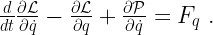
 , which is indeed volts.
 , which is also volts.
 , which is again volts (Ohm’s Law).
 or
or  has to be associated with each component of the system, and what voltages the
  correspond to. I think that will be easiest if I have some specific circuits to work with. Let’s start with a very simple one:
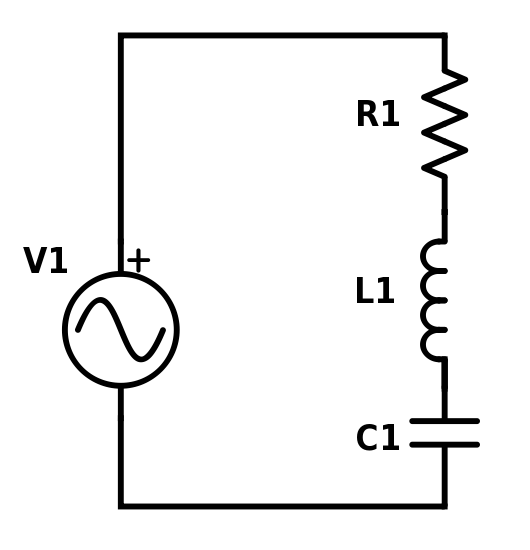
 , so that the current flow
  is clockwise in the schematic. We get the Lagrangian
 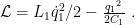 The power dissipation is
  , and taking the derivatives gives us
  , which is the voltage for the voltage source.
 , there is no kinetic energy (no inductors), and the dissipation is
  . Taking the derivatives of the Lagrangian gives us
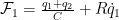 and
and .
. and
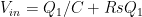
and  terms are 0 (modeling the voltmeter as a perfect infinite impedance), giving us the usual formulas for the input and output voltage, in terms of the charge on the capacitor:
 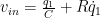 and
and  .
. and
and  , which gives us the transfer function
  , as expected. (Plug in
  to get the usual format in terms of angular frequency.)
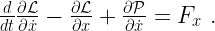
 , and the angle of the inverted pendulum (clockwise from upright)
  . The cart has mass
  and the pendulum
  , with a distance from the pivot on the cart to the center of mass for the pendulum
  . Furthermore, the pendulum has moment of inertia
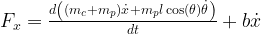
  , and there is viscous drag on the cart with a force
  . The pivot is assumed to be frictionless.
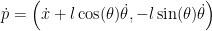
 to designate the location of the center of mass of the pendulum:
  .
. . The kinetic energy is
  . Combining these gives us
 .
. , and its square is
  . Substituting that into our previous formula gives us the Lagrangian in terms of just the generalized coordinates and their time derivatives:


 (the inverted pendulum straight up), by setting
  and
and  , except for the gravitational term, where we use
  :
:


")
 or hardback ($198)")

