Ultrasonic transmitter and receiver impedance measurement

In Ultrasonic rangefinder with Analog Discovery 2, I looked at the impedance of  an ultrasonic transmitter with the Analog Discovery 2, but I only modeled the transmitter as a capacitor, not modeling the resonances.

So today I collected new data, both for a transmitter and a receiver, using a 1nF C0G (1%) capacitor as the reference impedance, so that I could have clean data from a known pair.  I also looked at the transmitter+receiver as a network, and located the peaks of the signal transmission.  I was curious whether they corresponded more to transmitter or receiver resonances.

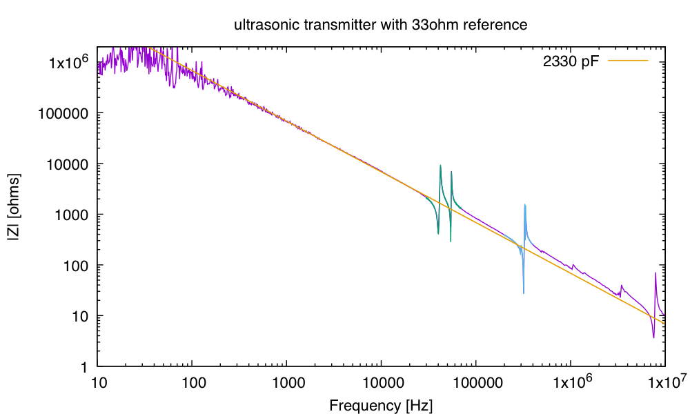
I could model the transmitter quite effectively as a capacitor with 4 LCR resonators in parallel.

I could model the receiver quite effectively as a capacitor with three LCR resonators in parallel.

The fitting was done with gnuplot, fitting one resonance at a time starting with the lowest frequency one, then refitting the previously fit parameters to tweak the fit. The radius of convergence for the fitting is pretty small—I needed to get the LC resonant frequency pretty close to correct before the fitting would converge. Increasing L makes the down-spike and up-spike closer together, and R controls how low the minimum gets, so I could get reasonable initial values (good enough to get convergence) without too much guessing, by plotting using the initial values, adjusting L to get the spacing between the spikes about right, adjusting C to get the resonant frequency right, and doing a rough guess that R is about the minimum value.

The peaks of the transmitter+receiver characteristic seem to correspond most closely to the minimum impedance points of the transmitter, which is reasonable when you consider that I’m driving the transmitter from a fixed voltage—the power is going to be V²/R, so power out is maximized when the impedance is lowest.  The one exception is the 331kHz peak, which seems to fall on the higher frequency of the two closely spaced transmitter resonances, and near the peak of receiver impedance. (Of course, only the 40kHz resonance of the transmitter or receiver actually gets used—the other resonances don’t provide nearly as much response in the transmitter+receiver pairing.)

Zooming in on the transmitter impedance for the high-frequency resonances, we can see that there are minor resonances that have not been modeled, but that the model does a good job of capturing the shape of the peaks. The peak of the transmitter+receiver response here falls on the higher-frequency resonance.

I did all my modeling with just the magnitudes of the signals, so it is interesting to see how well the model fits the phase response.

I got excellent matches to the phase response (even when I zoomed in on each peak), except for the low-frequency region, where the impedance seems to have a negative real part (phase < -90°).

I do have models for no resonance, single resonance, two resonances, and three resonances for the transmitter, as well as the four-resonance model. If a simplified model is needed, then it is better to take one of those fits, rather than omitting parts of the more complicated model, as each resonance affects the other parameters somewhat.
As a simple example, the receiver can be modeled as just a 739pF capacitor, but the LCR circuits contribute some of the capacitance, so 708pF gets used for the base capacitor of the model with the 3 resonances.

Ultrasonic rangefinder with Analog Discovery 2

In Loudspeaker impedance with Analog Discovery 2, I looked at the impedance of  various loudspeakers including an ultrasonic transducer. Today I looked at shaping pulse bursts for driving an ultrasonic transmitter to get shorter received pulses with an ultrasonic receiver.  I’ve done this before using custom programs on a Teensy 3.1 board (see Ultrasonic rangefinders arrived), but I wanted to see what I could do using just the waveform generator on the Analog Discovery 2.

I measured the magnitude of the impedance of the transmitter (using either a 120kΩ resistor or a 1nF capacitor as a known impedance), then looked at the transmitter+receiver characteristics for frequencies around the resonances.  I’ve marked the peak received resonances on the impedance plot.

The impedance is approx 2.2nF, with 3 apparent resonances.

The primary resonance is around 40kHz, and is the frequency that the transmitter is designed to operate at.

There is a secondary resonance around 54kHz, though it is considerably weaker than the 40kHz resonance.

The third resonance, around 330kHz does not provide a very strong signal for the receiver.

I tried two tests using the 40.445kHz resonance. In one, I used the simple waveform generator to produce a 40445Hz square wave, then used an 8ms wait and a 148.3µs run time, to produce bursts of 6 square waves. I set the idle output to the offset (0v) and used a 5V amplitude.

In the other test, I used the same wait and run times, but used the “custom” waveform to set up a signal that inverted the last 3 of the 6 periods (so that the half periods were +-+-+--+-+-+. This was fairly easy to set up by generating the 6 periods, then altering them by multiplying by a single period of a square wave. I could have created much more complicated bursts, but this pattern was enough to see the capabilities of the scope.

By triggering the scope on the signal sent to the transmitter (using channel 1), I could average 1000 sweeps to get a very low-noise view of the signal. (I can trigger on the waveform generator itself, freeing up one of the scope channels, but then I can’t average—I think that the averaging relies on interpolating get precise timing of the trigger.)  For plotting, I subtracted off the DC bias (fitted before time 0), as 60Hz interference caused a moderate offset to the signal even after averaging.

The bursts start out the same, but the simple 6-cycle burst results in the received waveform growing for 14 or 15 cycles, while the 3+,3- burst grows for 6–7 cycles and decays very quickly.

I tried some longer and shorter bursts, with the expected result that longer bursts resulted in stronger signals with a longer received burst width. Doing 8 cycles followed by 8 cancelling cycles seemed to produce a reasonable length burst with a fairly strong signal, but I did not explore variants much.

I still think it might be possible to use the phase information to get higher resolution than the approx 7.9mm wavelength, but identifying which pulse of the return waveform is which remains a problem, particularly if there is a complicated reflecting surface that superimposes several differently delayed pulses.

Loudspeaker impedance with Analog Discovery 2

One of the features of the Analog Discovery 2 that convinced me to buy it (rather than, say, a Rigol digital scope) was the ability to couple the waveform generator to the scope to do network analysis.  The basic idea of network analysis is to measure voltages at the output and the input of a 2-port network taking their ratio at different frequencies to get the response of the network.

Here is a generic 2-port network with a shared ground. If a sine wave is applied to the input, then the output will also be a sine wave (for a linear network) of the same frequency, but a different amplitude and phase.

If you model a linear system with complex numbers, then the output of any linear network driven by is , and the ratio of the output to the input is . A network analyzer drives a network with a succession of different sine waves, recording the amplitude ratio and the phase shift $\phi$ for each frequency.

I haven’t often needed a network analyzer, but I have many times done something very similar: impedance spectroscopy, which looks at the ratio of the voltage to the current at different frequencies. The loudspeaker and electrode labs in the course both do this, but only recording the amplitude ratio, not the phase change, as hand measurements with voltmeters do not provide a way to determine the phase.

Because the network analyzer just takes the ratio of Channel 2 divided by Channel 1 and both are differential input channels, we can use it as an impedance spectrometer.  We just put the device under test (DUT) in series with a known impedance (comparable to the one to be measured), drive the series chain with the waveform generator, and measure the voltage across the two impedances.  We then have .

For example, here is the result of running the network analyzer for an 8Ω loudspeaker with a 33Ω known impedance:

At frequencies above about 1MHz, I don’t believe that the test setup is really measuring the behavior of the loudspeaker.

For impedance spectroscopy, the default display with the amplitude in dB is not particularly friendly, so I saved the data, fitted a model to it with gnuplot, and plotted it:

Loudspeaker model to fit.

Amplitude data and fitted model. Note that the impedance does not rise as fast as a simple inductor for L1 would imply.

Compare the plot above with the hand-measured ones at Better model for loudspeaker or Loudspeaker analysis.  We can see the limitations of the model even more clearly when we look at the phase change:

At low frequencies, the model and the measurements fit well, but at high frequencies, the phase only goes to 50°, not 90° as would be expected of an inductor.

I also measured a tiny 8Ω loudspeaker that I had bought to experiment with ultrasonics (see Redoing impedance test for tiny loudspeaker):

The main resonance around 1390Hz is clearly visible, but there appear to be some higher resonances as well.  We can do a more focussed sweep to see them clearer:

The secondary resonance peaks are clearly visible when we scan a narrower range.

The model for the tiny loudspeaker fits the phase measurements better than for the larger loudspeaker, but the phase still only gets to 66°, not 90°.

I also tried one of the ultrasonic transmitters (see Ultrasonic transmitter impedance again for hand measurements):

With a 33Ω current-sense resistor, the low frequency end of the impedance spectrum is just noise—there is almost no voltage drop across the 33Ω resistor.

Using 1nF capacitor as a reference impedance, rather than a resistor, results in much more comparable voltages across the whole frequency range, and a cleaner impedance spectrum. But at low frequencies, we’re really seeing the impedance of oscilloscope inputs, rather than the ultrasonic transmitter.

For the piezoelectric ultrasonic transducer, the phase spectrum is easier to see the resonances in.

There are some high frequency resonances as well as the main ones.

I also tried using the network analyzer as a proper network analyzer, where the network consisted of the tiny loudspeaker acoustically coupled to  an electret microphone which had a 10kΩ pullup to 5V:

The 9.5–10kHz peak was distinctly audible (even though I’m rather deaf in that range), so the resonance was in the loudspeaker not the microphone.

I get somewhat different results with the larger 8Ω loudspeaker:

I have a much more uniform response across frequencies, but it looks like I get a fairly strong response even at very high frequencies. I wonder if I’m seeing an electrical rather than acoustic coupling.

Finally, the ultrasonic transmitter:

With a 2V amplitude (instead of 500mV) I get a smaller signal from the ultrasonic transmitter. There does not seem to be a peak at 40kHz, where the transducer is normally used.

There is an antiresonance around 39kHz and a resonance around 54kHz. Perhaps it would be better to use the transmitter at 54kHz than at the normal 40kHz!

Redoing impedance test for tiny loudspeaker

In Ultrasonic rangefinder tests with tiny loudspeaker, I tested the 10mm CDM-10008 loudspeaker and found it ringing around 9.4kHz, but I reported

I don’t see any resonance around 9.4kHz in the impedance plot, though I admit not looking for narrow resonance peaks in that range.

Today I redid the impedance tests using a 10Ω sense resistor, so that I could use the same range for all voltage measurements, resulting in more correct impedance measurements.  I could definitely hear a resonance around 9.5kHz (and given my deafness at high frequencies, it must have been very loud indeed for me to hear it so clearly), so I looked for another peak in that neighborhood.  It is there and measurable, but not very prominent in the plot:

Because the second peak is on the sloping part of the plot and quite small, I had to model the loudspeaker with a j ω^α L semi-inductor to get a good fit.

I have not attempted to fit the data points past 200kHz, because I don’t believe that the multimeter I was using is really good at those frequencies.  The “corner frequency” I’m reporting around 100kHz is where the DC resistance is equal in magnitude to the impedance of the semi-inductor.

Given how small the peak is on the |Z| graph, but how loud the sound is around 9.5kHz, I probably need a different way of looking for resonances beyond the main one. I can’t rely on my ears for loudness at high frequencies, but perhaps I could use a microphone and record the amplitude it sees as a function of frequency.

Ultrasonic rangefinder tests with tiny loudspeaker

I’m still working on doing the ultrasonic rangefinder project  (In More testing for ultrasonic rangefinder, I gave a digital filter and showed it working with a non-resonant electret microphone and amplifier and pings from a Maxbotix rangefinder.  In Ultrasonic rangefinders arrived, I looked at generating good 40kHz pings while listening to the direct sound with a microphone and amplifier. In Ultrasonic rangefinder without amplifier, I tried seeing if we could use the transducers without an amplifier. In Ultrasonic rangefinder with loudspeaker, I tried using a midrange loudspeaker to generate the pings (but was limited to about 20kHz.)

For the past couple of days I’ve been working with a tiny (10mm) loudspeaker, to see if I could get to higher frequencies without a resonant transducer, so that I could play with doing spread-spectrum pings that can be deconvolved to get more precise and more accurate measurements of echoes. I expected the 8Ω loudspeaker to be much less efficient than a resonant transmitter, but beyond that I had few preconceived notions of how well it would work.

Here is the front of the CDM-10008 10mm loudspeaker.

Here is the back of the loudspeaker, with the two solder points visible on the bottom.

Soldering the leads on was more difficult than I expected. I started out putting the loudspeaker face down on the bench and approaching it with the wire and soldering iron, but the loudspeaker jumped off the bench and stuck to the iron—I’d forgotten that the soldering iron tip really does contain iron, and that the magnet for the tiny loudspeaker is unshielded. After sticking the loudspeaker into a Panavise board holder, I had no trouble soldering on the leads.

Here is the loudspeaker with wires soldered on, and a female header with some double-ended male header pins to make it easier to attach to a breadboard.

The first thing to do (after checking that the leads weren’t shorted) was to measure the impedance as a function of frequency, using a voltmeter, a 100Ω series resistor, and a function generator. I was working at home, so I used a Fluke 8060A multimeter that I bought used on e-bay (which replaced my old 8060A that had failed). Unfortunately, the “new” meter is not much better, as the different voltage ranges seem to have radically different calibration. I used one range consistently for the loudspeaker voltage, and another consistently for the resistor voltage, so the shape of the curve should be ok (up to 300kHz), but |Z| may need to be shifted up or down by as much as 20%.

The resonant peak at 1340Hz is consistent with the datasheet, which specifies 1200Hz with a range from 960Hz to 1440Hz. They specify the power output for the speaker in the range around the resonant peak, which gives an exaggerated view of the response elsewhere.

I tried driving the loudspeaker directly from pins 16 and 17 of the Teensy LC, which I had configured for high drive, with the setup() routine containing

    CORE_PIN16_CONFIG |= PORT_PCR_DSE;
    CORE_PIN17_CONFIG |= PORT_PCR_DSE;

I also put a 10Ω resistor in series with the 8Ω loudspeaker, to limit the current demanded of the I/O pins (though still far more than they are supposed to deliver). With this setup I got about ±1.6V between the pins, ±860mV across the resistor (so ±86mA), and ±670mV across the loudspeaker. The loudspeaker voltages showed spikes, but the resistor voltages were fairly clean square waves, even with 100kHz square waves.

I then made an amplifier for the electret microphone, keeping the gain per stage low to avoid the 1MHz gain-bandwidth limit of the MCP6004 op amps. With a gain of only 10 per stage, I should have a bandwidth close to 100kHz.

Here is the schematic for my test fixture. I looked at the microphone and speaker signals with both my Bitscope oscilloscope and at the microphone signals with the Teensy ADC.

I started out looking a some complicated pulse patterns that I had designed to have high energy in the 20kHz–50kHz range, but a low autocorrelation other than at 0s. These pulse patterns should be good for the spread-spectrum tests I wanted to make. I was disappointed, however, in not being able to see the patterns in the recordings from the microphone, so I switched to a simpler stimulus—a single short pulse.

Short pulses seemed to trigger a resonance in the loudspeaker at about 9.4kHz, though short pulses resulted in an initial higher frequency mode being excited.

Each of the plots were made by averaging about 3 dozen traces recorded by the Teensy, to reduce noise. I found that I had to unplug the power supply from the laptop that was providing the USB power, as I otherwise got a lot of 90kHz noise.

I don’t see any resonance around 9.4kHz in the impedance plot, though I admit not looking for narrow resonance peaks in that range. I was a little worried that it might be related to the high-pass filters in the amplifiers which had a corner frequency near there, so I redid the tests with different filters, changing the 330pF to 680pF, so lowering the corner frequency to 4590Hz. The impulse response is much the same:

The signal is a little stronger with the high-pass having a lower corner frequency, but otherwise not changed much.

Note: the signal visible before the sound arrives is probably due to electrical noise from the loudspeaker coupled through the power supply,as it appears as the pulse is shut off.

Unfortunately, this little loudspeaker does not seem to be usable for the spread-spectrum sound production that I had hoped for, as the 9.4kHz ringing is definitely going to corrupt any high-frequency waveform I try to impose.

The ringing the loudspeaker is larger than for the ultrasonic transducer, so we’re actually getting more sound, but the transducer takes much less current, and I’ve not attempted to compare efficiencies.  Both ring for 1–1.5ms, which is too long for what I wanted to do.