Second half of temperature lab went well

I continue to be pleased with this Spring’s class.  It is taking up far too much of my time, but the students are doing well. Today they got their resistors (and ceramic capacitors), so they could select whatever resistor value they needed for the optimization problem.  I told them by e-mail last night to optimize for 12°C, which I estimated would require about a 12kΩ resistor.  I change the temperature point each year, so that students can’t just look up an answer—not that it would do them much good if they could, as the design report needs to contain the derivation of the result.  If they can copy the math correctly, then they can do it (especially since we did the derivation in class yesterday).

I put some reminders/instructions on the board at the beginning of lab, something like the following:

• Optimize for max sensitivity @ 12°C
• Measure your resistor
• Measure Vin
• Measure Vout at many temperatures
• Plot Vout vs temp both from model (as curve) and as data points, to check calibration.
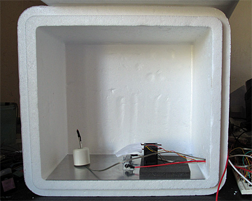
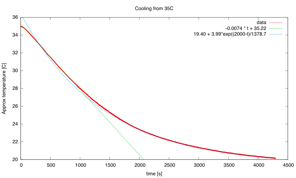
• Plot temp vs time for 10 minutes of water warming up from low temperature (using PteroDAQ)

Everyone seemed to be getting good data in the lab.  What students seemed to need the most help with was the concept of putting the predicted behavior of the circuit on the same graph with the measured behavior. They had a formula for the voltage as a function of temperature with 4 parameters: B and R∞ from fitting Tuesday’s data, R that they chose and measured, and Vin that they measured though it was nominally 3.3V. But it was hard going trying to convince them to plot that curve on the same graph as the scatter diagram of today’s measurements.  It may be that they have never been asked to plot a predicted curve and measurements on the same plot before—as if they’ve never actually checked that a model is correct. I would have thought that physics classes would have done that sort of predictive modeling, but apparently not, as the concept seemed completely foreign to many of the students.

Those who did finally get the calibration plot done generally had very good agreement between their measurements and the predicted model.  I’m hoping the rest will get the plots done tonight.  There was at least one group that was seeing about a 0.5°C discrepancy, which could be due to different calibration of the thermometers used on Tuesday and today, or could be due to their using a wrong value for the °C to °K conversion.

The students also recorded a time course of a water bath warming up from about 3°C. I think that next year I might do a higher optimum temperature and ask students to record a water bath cooling down—the temperature change is faster that way (due to evaporation). I’ve asked them to plot this as temperature vs. time, not voltage vs. time, and several students seemed well on their way to doing that correctly—this year’s class seems much more adept at picking up gnuplot techniques than the last two years’ classes.  I don’t know whether that is because of a better ordering of the material this year, or some difference in the cohort.  I like to think it is an improvement in the way I present things, but it is more likely to be a difference in the students.

One pair of students surprised me in a good way—they had done the optimization last night, then tried out the design at home, using the PteroDAQ to read voltage.  Since they did not have the resistor kits yet, they had put the two 22kΩ resistors they did have in parallel to make an 11kΩ resistor.  They were worried I might be upset with them for jumping the gun on the lab—quite the contrary, I’m delighted that they’re preparing before class, and that they realized that a lot of the lab work doesn’t really require the fancy equipment in the lab. I’ve pitched the class as being suitable for creating electronics hobbyists, and if some of them get into that early in the course, then the course is being highly successful!

I’ve even considered rewriting a number of the labs to be doable completely at home, but right now too many would require about a $250 investment in a USB oscilloscope, which makes an all-at-home approach a bit too expensive for me to recommend.  It might be an interesting way to market the book though—as a complete electronics at home lab course for about $400.  I think that there is a substantial market for such a kit/course, but it would be a fair amount of work to get the book into shape for use without a lab mentor to guide the students through the rough spots.

I’m looking forward to this week’s reports (that’s right, for once I’m looking forward to the grading, rather than dreading it), as I think that a lot of the class actually got all the concepts that this week’s lab was about.

Tomorrow I’ll be introducing complex impedance (particularly ) and RC filters as voltage dividers.  I’ll be doing most of the lecture as a chalk talk, but I’ll bring my laptop to show them how to create (amplitude) Bode plots with gnuplot.  We’ll be doing various things with model fitting, with variants on voltage dividers, and with complex impedance for the next 3 weeks, and then we’ll start on amplifiers.

 

 

Optimization and model fitting went well today

Today’s lecture in BME 101 (the Applied Electronics for Bioengineers class) went very smoothly. I started with a little light entertainment: a video about blowing up capacitors, sent to me by Jameco: http://www.jameco.com/Jameco/content/incorrectly-using-capacitors.html This video reinforced the message that I had given them in lab last week about electrolytic capacitors.

I had two topics to cover: the optimization problem from last weekend’s homework, which only one student had managed to do, and model fitting to extract parameters for the thermistor model from the data collected in lab yesterday.

I gave the students the choice of order for the topics, and they wanted the optimization first.  The problem is fairly straightforward from an engineering standpoint: we want to maximize the sensitivity of the circuit that converts temperature to voltage at a specific operating temperature T_opt. I first sketched very rough plots of what the voltage would look like as a function of temperature: monotone increasing but not particularly linear. I reminded them that sensitivity is the change in output that you get for a given change in input: dV/dT.  I coaxed out of the class the idea that to maximize the function dV/dT, we need to take its derivative and set it to 0: .  We only have one free variable in our circuit to change (the load resistor R), so we need to take that equation and solve it for R, to get the value of R that maximizes sensitivity.

I reminded them of the simple model for the resistance of a thermistor that we’d had on Monday: , and they had no trouble coming up with the equation for the output voltage .  I then suggested using Wolfram Alpha to solve the equation, and switched from the chalkboard to the screen to type

solve d^2 (R/(R+S e^(B/T)))/ dT^2 = 0 for R

(changing R_∞ to S, to avoid confusing Wolfram Alpha with subscripts).
Wolfram Alpha conveniently replied with two solutions: R=0 (which would result in a constant 0 output voltage, clearly a minimum sensitivity) and . I pointed out that the first part was just the resistance of the thermistor at the temperature we were optimizing for, and the second term scales that down a little.

We then moved on to fitting the model. I showed three data sets that students had sent me—one which was a little messy, but still quite usable, one that was a little better, and one that was really beautiful.  I continued with the really good data set.  I explained that gnuplot tries to minimize the error on the y-axis for a function of things on the x-axis, and the students decided that minimizing the temperature error for a given resistance was probably best here. (I suspect it doesn’t make much difference with this data, but it is good to get them to think about that as a decision that needs to be made for each modeling problem.)

On the board, I turned around the equation for the model, to get temperature in terms of R: .

I then developed the gnuplot script for the problem live, debugging as I went.  Some of the errors to debug were ones I introduced deliberately, others were inadvertent, but all were good for teaching both the process of debugging and the notion of doing sanity checks.  My first mistake was an inadvertent one: I capitalized a variable differently in the parameter list and in the function body, and gnuplot is case-sensitive.  This was very easy to find and fix, and gave me an opportunity to tell students that gnuplot was sensitive to case, since that had not come up previously. My second mistake was a deliberate one: I typed in the model exactly as we had derived it on the board, knowing full well that the model was for °K, but the data was for °C.  I’d even reminded students of that earlier, when we were doing the optimization problem.

I then ran the fit in gnuplot and asked students if we were done, or if there was a sanity check we could do.  A couple of them asked if we could plot the model and the data on the same plot, so I did that. The fit was very obviously completely wrong. So I asked the students what was wrong and how we could fix it. I did dice-assisted cold calling to put 3 or 4 students on the spot, getting not very useful answers, then took answers from a couple of students who raised their hands. The second student pointed out the °C vs °K problem.

So I fixed the formula and ran the fit again, expecting everything to work fine.  It didn’t! So we went into debugging mode, trying to see if starting with better estimates of B and R_∞ would help. Nope. Then I realized that I had made a second inadvertent error: I’d put in 273.15 with the wrong sign! I fixed that, ran the fit again, and again things failed (producing negative values for R_∞).  This time, though when I put in better initial estimates, everything converged to a very good fit, which gave me a teachable moment about the need to have decent estimates before fitting, so that the optimization algorithm that did the fitting could converge.

The final script was

temp(R,B,Rinf) = B / ( log(R) - log(Rinf)) - 273.15
B=3000; Rinf=1e-4
fit temp(x,B,Rinf) 'student-thermistor-data-3.txt' using 2:1 via Rinf,B
plot 'student-thermistor-data-3.txt' using 2:1, \
      temp(x,3435,10*exp(-3435/(25+273.15))), \
      temp(x,B,Rinf)

The second curve of the plot is using the data sheet values for the B value and for R_25°C=10kΩ.
Here is the plot produced:

Notice that I did not have axis labels, title, nor echoing of the parameters in the key. We covered that last week and I’m hoping that students can carry skills over from one week to the next.

The model fit is slightly better than the data sheet values, but the data sheet values were closer than I had expected based on previous years’ fits. I think that it may be that the students had a properly calibrated thermometer (I’d removed any digital thermometers that reported ice water as warmer than 0.5°C—about 1/3 of them were that far out of calibration), and that this particular pair of students had been very careful with their measurements.

Temperature lab went well

The lab for characterizing the thermistors went well—more smoothy than the last two years.  It may be because the lab is now in the second week, rather than the first week, or it may be because I required prelab homework be turned in on Monday, so that students came to lab already prepared, or it may just be that this year’s class is more prepared than previous ones.  I suspect that the main difference is in the prelab requirement, but that may be because that is about the only thing I can really control.

I went into the lab an hour early, to set up the coffee urn with hot water, get ice from the ice machine in the lab upstairs, and check each of the thermometers in ice water.  The cheap student glass thermometers all ready between -1°C and 0°C, but several of the digital thermometers were way off (reading as much as 4°C).  I separated out the digital thermometers that read over 0.5°C and marked them with blue tape as miscalibrated.  (I can believe temperatures slightly below 0°C, since the ice water was tap water, not distilled water, but temperatures over 0°C were almost certainly wrong.)

I started by showing the students how to interpret the part number for the NTCLE428E3103F520L thermistor we were using, since half the class had not figured out that it was a 10kΩ thermistor on the homework.  The data sheet is rather tricky, but in a common way: it is the data sheet for a family of parts, with a key for decoding the part number.

The students managed to collect 20–90 data points of temperature and resistance, with varying levels of noise.  I had them plot the data after they had collected some points, and suggested to students that they fill in more points where they had gaps in the curve, or where they had “bumpy” spots that did not fall along a smooth curve (suggesting measurement errors), and pushing them to get lower and higher temperature measurements.  Students with good lab skills managed to get a lot of data points from 2°C up to 69°C.  The water in the coffee urn was a bit hotter than that, but by the time they got the water back to their benches and made measurements it had cooled off.  It might be interesting some year to have a hot plate at every bench to let them measure up to 100°C, but I don’t think that the expense of the hot plates would be justified for this one lab—and I’d worry about possible spills.

I was worried enough about spills on this lab, reminding students frequently to carry the secondary containment tubs in both hands, and to put it flat on a level surface whenever they weren’t carrying it.  As it turns out, about the only real spill was mine, trying to pour ice water from one thermos to another, and getting a chunk of ice splashing out.  The spill was small (a few cubic centimeters of ice) and not near the lab equipment, and I could mop it up with a couple of paper towels. I was probably made a bit clumsier than usual by having only gotten 4 hours sleep last night (between grading prelab homework and adding material and exercises to the chapters of the book that the students need to read for Friday and next Monday).  Still I felt bad about being the clumsy one in the room.

There were two glass thermometers broken—one was taken in its case by a student to be properly discarded in a broken-glass disposal bin, but the other was just quietly returned to the bin of thermometers.  I have a lot more respect for the student who reported the broken thermometer than the one who tried to hide it.  The thermometers themselves are cheap (about $3), so the breakage doesn’t bother me, but leaving problems for someone else to deal with does.

I had a few of the students send me data, which I will use in class today to show students how to use gnuplot to fit models to data. I also plan to go over the homework problem that only one student got—the optimization to maximize the sensitivity of the voltage divider at a particular operating temperature.

 

Thermal control loop working (sort of)

Classes start tomorrow, so I spent yesterday making sure that the incubator control project was feasible. I had gotten the fan feedback control working well back in September, but I’d put the project aside for Fall quarter and only got back to it this week.  As a reminder, here are the previous posts on the project:

• Temperature-control project for freshman design seminar describes an idea for a possible project for the freshman design seminar.
• PWM for incubator gives a bit more detail on the temperature-control project.
• More on incubator design continues the incubator design.
• Thermal models for power resistors presents thermal models for 3 power resistors without heatsinks.
• Thermal models for power resistor with heatsink applies the simple thermal model to a power resistor with a heatsink, where it does not fit quite as well.
• PWM heater and fan talks about doing PWM for a fan and for a resistor as heater.
• PWM heater and fan continued continues the previous design work, reducing the electrical noise and making PI control loops for the fan and the heater.
• Controlling the heater and fan talks about progress on the control loops and gives the schematic for the circuit discussed in the two previous posts.
• Putting the heater in a box shows the physical layout of the partially completed incubator and discusses the (meager) progress today.
• Improving feedback for fan shows the working control loops, and compares on/off, hysteresis, PI, and PI with anti-windup.

Here is the interior of the styrofoam box, with the lid open. The 6″×12″ aluminum plate covers the bottom. The thermistor is on the left, propped up by a rubber foot, the resistor in is the center, and the fan is sitting on a foam pad on the right. (The foam is to reduce noise until I can get the fan proper mounted in a baffle.)

I left the foam out this time, which made for a somewhat noisy fan, and I still haven’t built a baffle—I’m still using the bent-wire-and-paper deflector shown in the photo. What I worked on yesterday was the software—since the temperature changes are fairly slow, it takes a long time to tune the control loops.

One thing I did was to try to reduce measurement noise further on the thermistor measurements. I now add 60  analog-to-digital readings. They’re 10 bits on the Arduino-compatible board (a Sparkfun redboard), so adding 60 still fits in an unsigned 16-bit word. I now get noise of about ±0.05°C, which is half the least-significant-bit of the converter.  I doubt that I can do better in precision without switching to a processor with a better analog-to-digital converter, though I could do digital filtering with a 1Hz low-pass filter to smooth out the remaining noise.

I copied the fan feedback control loop (with the anti-windup provisions) described in Improving feedback for fan for temperature control, but made two changes:

• I changed the integration time and K_p for the thermal control loop, since the temperature response is much slower than the fan response.
• Because of the huge asymmetry in the temperature response (the resistor and metal plate can heat up much more quickly than they cool down), I turn off the heater the moment it gets over temperature, no matter with the PI loop suggests, but I only switch to full-on when the air temperature is 3°C too cold. For the fan, I used a symmetric window around the set point for using the PI loop rather than full-on/full-off.

Here are some results from tuning experiments:

The blue curve switched to PI control at 23.5°C, the other two at 22°C. The green curve has pretty tight control over the temperature, but does overshoot a bit.

The initial temperatures were not all identical, because I wasn’t always willing to let everything cool down all the way to room temperature after each tuning run. I could only do about 1 tuning run an hour, which could pose problems for the freshman design seminar, as we don’t have long lab times—only the 70-minute lecture-schedule meeting times.

I continued the best of those runs with another step, up to 35°C, then let it cool down.

The step to 35°C has more ringing than the step to 25°C. I terminated the run before it had finished cooling, because the 32-bit µs timer wrapped around.

The cool-down at the end fits a 0.0069 °C/s line better than it fits an exponential decay to the ambient temperature.  If I do fit an exponential decay curve, I get a time constant of around 1975 seconds.

A simple thermal-resistance, thermal-capacity model is not a very good one for predicting how the system will behave, particularly since we’re not measuring the temperature of the large thermal mass (the aluminum plate and power resistor), but of the air, which has a large thermal resistance from the plate.  The time constant for the aluminum-air transfer is larger than the time constant for the electricity-aluminum transfer, which is why we get so much overshoot when we turn off the power to the resistor—the aluminum plate has gotten much hotter than the air, and continues to transfer heat to it, even though no more heat is being added to the aluminum.

Still, it is worth seeing what we get if we model the box a simple thermal mass and thermal resistor. The steady-state 35°C seems to need about 9W (PWM of 51/256) and the 25°C 3W (PWM of 17/256) with an ambient temperature of about 19°C, implying that the styrofoam box has a thermal resistance of about 1.9°C/W.

To see what is really going on, I’ll have to heat the box to 35°C, then start the cool down with a reset 32-bit timer.

Single-step warming from 16.9°C to 35°C. The steady state at 35°C is about 9.32W, for a thermal resistance of 1.8°C/W. The rise of 0.0451°C/s at 45W implies a thermal capacity of 998 J/°C.

Heating at 45W (9V, 1.8Ω) results in a temperature rise of about 0.0451 °C/s. This warm-up rate at 45W implies a thermal capacity of about 998 J/°C. We may want to adjust our thermal capacity estimate, since some of the 45W put in escapes through the box—maybe about 3–4W at the temperatures where the rise was measured. This reduces the thermal capacity estimate to about 910 J/°C.

The cool down from 35°C starts out as a straight line (about -0.0074°C/s or -26.5°C/hour), but gradually starts behaving more like the exponential we would expect from a thermal-resistance and thermal-capacity model.

The time constant for the cooling is about 1380s, but the initial cooling is too slow for a simple exponential.

The time constant of 1380 s, combined with a thermal capacity of 910 J/°C gives a thermal resistance of 1.5 °C/W, a bit lower than the 1.8°C/W I estimated from the steady-state power.

I continued the cooling (with the timer wrapped around) to see if I got a clean exponential at low temperature differences:

The exponential seems to fit well here, with a time constant of 2300s. Combined with the 910 J/°C, this gives a thermal resistance of 2.5°C/W, which seems a little high compared to the other estimates.

So I’ve made some progress on the thermal control loop (though I’d like to reduce the overshoot and ringing) and I have a crude model for the box: a thermal mass with capacity about 910 J/°C and thermal resistance 2±0.5 °C/W.

Still on my to-do list for this project:

• Consider using a PID controller for the temperature to get faster response without overshoot.  (If I can reduce the noise problem.) I should be able to reduce the noise with a digital filter, but I’m already pushing well beyond what I’m comfortable covering in a freshman class. Tuning a PID controller is even trickier than tuning a PI controller, which is already going to take most of the quarter to teach.
• Design and build baffling for the fan to get better airflow in the box. This might be a good thing to get students to do, particularly if we can get them to learn how to use the laser cutter. But even handsaws would suffice, given some thin plywood or masonite, some angle irons, and nuts and screws.
• Figure out how to get students to come up with workable designs, when they are starting from knowing nothing. I don’t want to give them my designs, but I want to help them find doable subproblems. Some of the subproblems they come up with may be well beyond the skills that they can pick up in the time frame of the course. The more I work on this project, the more I realize that I and the students will have to be happy with them having explored the options, without getting all the problems solved.
• Add changes to the cumulative error term whenever K_P or T_I are changed, to keep the PWM output the same after the changes—currently changing any of the control loop parameters adds a huge disturbance to the system. I don’t know how important this is—I’ve been doing my tuning of the thermal loop by recompiling, rather than by changing parameters on the fly. The quick changes were handy for the fan loop, where I could see things happening quickly, but for the thermal loop each experiment took about an hour, so there was no need for a fast parameter change.
• Research control algorithms other than PI and PID, particularly for asymmetric systems like the temperature control, where I can get fairly quick response to the inputs when heating, but very slow response when cooling. The asymmetric window for switching between on/off and PI control seems to have helped here, but there is probably a more principled way to handle asymmetric control inputs. Maybe I should ask some of the control-theory faculty for some pointers.
• Develop a more detailed thermal model with separate components for the aluminum plate and the air in the box. It may be worth adding another thermistor, taped to the aluminum plate, to monitor that temperature. The extra thermistor would also allow much tighter temperature control, avoiding overshoot on air temperature.

 

Putting the heater in a box

Continuing the saga of the incubator project in the recent posts:

• Temperature-control project for freshman design seminar describes an idea for a possible project for the freshman design seminar.
• PWM for incubator gives a bit more detail on the temperature-control project.
• More on incubator design continues the incubator design.
• Thermal models for power resistors presents thermal models for 3 power resistors without heatsinks.
• Thermal models for power resistor with heatsink applies the simple thermal model to a power resistor with a heatsink, where it does not fit quite as well.
• PWM heater and fan talks about doing PWM for a fan and for a resistor as heater.
• PWM heater and fan continued continues the previous design work, reducing the electrical noise and making PI control loops for the fan and the heater.
• Controlling the heater and fan talks about progress on the control loops and gives the schematic for the circuit discussed in the two previous posts.

On my to-do list for the project

• Put the whole thing into a styrofoam box, to see whether extra venting is needed to allow things to cool down, and to see how tightly temperature can be controlled. Find a smaller bread board or prototype board to put the controller on—my current bread boards are all 6.5″ long, and the box only has room for 6″, especially since I put the resistor in the center of the 6″×12″ aluminum plate, which just fits the box. I suppose I could drill a couple more holes in the plate and mount the resistor off center, but I rather like the idea of building the controller as an Arduino shield, so that the Arduino + controller is a single unit. Another possibility is to drill a hole in the styrofoam box and run cables through the box for the resistive heater, the fan, and the thermistor. Even if the grounds are connected outside the box, this is only 8 wires. Putting the control electronics outside the box would reduce the clutter in the box and make tweaking easier
  

  I got this done today, by drilling a hole in the box and soldering long wires onto the resistor and the thermistor, so that all the active electronics could live outside the box. Incidentally, “drilling” did mean using a drill bit, but I held it and turned it with my fingers—styrofoam is so soft and grainy that I feared a power drill would tear out big chunks.

  

  Here is the interior of the styrofoam box, with the lid open. The 6″×12″ aluminum plate covers the bottom. The thermistor is on the left, propped up by a rubber foot, the resistor in is the center, and the fan is sitting on a foam pad on the right. (The foam is to reduce noise until I can get the fan proper mounted in a baffle.)

  As expected, I can heat up the thermistor fairly quickly, but if I overshoot on the temperature, it takes a very long time for the closed box to cool back down. Cooling off just 1°C took over half an hour.

• Add some low-pass filtering to the temperature measurement to reduce noise. Just adding 4 measurements in quick succession would reduce the noise and give the illusion of extra precision.

  I did this also. With the box closed, the thermistor reading is fairly stable, with fluctuations of less than 0.1°C (which was the resolution with a single thermistor reading before adding 4 successive reads).

• The fan controller occasionally has a little glitch where the tachometer either misses a pulse or provides an extra one (I think mainly an extra one due to ringing on the opposite edge).  I could try reducing this problem in three ways: 1) changing which edge I’m triggering on, 2) using more low-pass filtering before the Schmitt trigger in the edge detector, or 3) using median filtering to throw out any half-length or double-length pulses, unless they occur as a pair.  (Hmm, the half-length pulses would occur as a pair, so this might not help unless I go to median of 5, which would be a lot of trouble.)

  I fixed this also, using two techniques:

  1. In the program I have 3 states for the interrupt routine that catches the edges: normally, I check that the edge is within 3/4 to 3/2 of the previously recorded pulse—if so I record it and continue. If it is less than 3/4 as long, I skip it, and change to a skip state. If it is more than 3/2 as long, I skip it and switch to a force state. In the skip state, I ignore the reading and switch to the force state. In the force state, I accept the pulse length (whatever it is), and switch to the normal state. With this state machine, I ignore a double-length pulse or a pair of half-length pulses together.
  2. The rising edge of the pulse from the tachometer is very slow (thanks to the RC filter of the pullup), but the falling edge is sharp. Extraneous pulses are more likely to occur if I trigger on the slow edge rather than fast edge, so I switched the polarity to make sure that I was using the falling edge (which is the rising edge of the output of the Schmitt trigger).

  I think that changing which edge I used made a bigger difference than trying to suppress the erroneous reads digitally. I no longer hear the occasional hiccup where the control algorithm tries desperately to double or half the fan speed because of a misread timing pulse.

• Improve my anti-windup methods for both thermal and fan controllers, to reduce overshoot.

  I changed from using conditional integration and back calculation of the integration error to using a decay of the integration error based on the difference between the computed PWM setting and the limit when the limits were exceeded. I’m not sure this improved anything though, and it introduces yet another parameter to tune, so I may go back to the previous method. I did play around with the tuning parameters for the fan loop today, and realized that I still don’t have good intuition about the effect of parameter changes. I noticed that the fan control was oscillating a little (small fluctuations around the desired speed, but big enough that I could hear the changes), and I found ways to reduce the oscillations, but at the expense of slower response to step changes.

• Improve my modeling of the thermal system, so that I can do more reasonable back calculation on setpoint change.

  I still need to do more thinking about the thermal modeling, since it is clear that I can’t afford overshoot when heating (though overshoot during slow cooling is unlikely to be a problem).

Still on my list with no progress:

• Consider using a PID controller for the temperature to get faster response without overshoot.  (If I can reduce the noise problem.)
• Design and build baffling for the fan to get better airflow in the box. I’ve made a little paper and wire baffle, to get better air flow over the resistor, but I’ve not done the full baffling to get good airflow in the box.
  
• Figure out how to get students to come up with workable designs, when they are starting from knowing nothing. I don’t want to give them my designs, but I want to help them find doable subproblems. Some of the subproblems they come up with may be well beyond the skills that they can pick up in the time frame of the course. The more I work on this project, the more I realize that I and the students will have to be happy with them having explored the options, without getting all the problems solved.
  

I want to add to the list today:

• Add changes to the cumulative error term whenever K_P or T_I are changed, to keep the PWM output the same after the changes—currently changing any of the control loop parameters adds a huge disturbance to the system.
• Separate the control algorithm better from the rest of the code, so that I can use the same code base and quickly switch between different control algorithms: on/off, on/off with hysteresis, proportional control, proportional control with offset, PI control, PI control with anti-windup variants, PID control.
• Add an option for recording the response of the system over a long time, so that I can plot input and output of the system with gnuplot. This would be nice for the fan control loop, but I think it will be essential for the temperature control loop.
• Research control algorithms other than PI and PID, particularly for asymmteric systems like the temperature control, where I can get fairly quick response to the inputs when heating, but very slow response when cooling.