Gas station without pumps

2022 March 29

Better heartbeat detection

Filed under: Circuits course — gasstationwithoutpumps @ 14:37
Tags: , , , , ,

In Lower PVC frequency, I promised “I’ll report on the algorithms when I get something a little better than I have now.”

I’ve played with three algorithms this week:

  • Doing spike detection, then measuring the time for 2n periods by looking at the time between the spikes n before andafter the current spike.  This gives a fine resolution both in time and frequency, and provides smoothing because adjacent measurements overlap by 2(n-1) periods. It is, however, very susceptible to errors due to miscalling the spikes.  Missed spikes result in too low a frequency, and extraneous spikes result in too high a frequency. I could increase n to reduce the effect of miscounts, but at some loss of time resolution when pulse rate changed.
  • Taking FFT of a block of samples (say 4096, which is about 17 seconds at 240 Hz) and looking for a high energy frequency.  Temporal resolution is poor (even with 50% overlapping blocks we get one measurement every 8.5s) and frequency resolution also poor (bins are about 3.5 bpm wide). I tried improving the frequency resolution by looking at the phase change for the peak between adjacent windows, but that didn’t solve the main problem, which was that choosing the right peak in the spectrum was often difficult.  The simple algorithms I tried for choosing the peak often failed. I eventually gave up on this technique.
  • Taking the autocorrelation of a block of samples (using rfft and irfft) and looking for a peak. The time for that peak is the period, which can be inverted to get the frequency.  This method provides the same coarse time resolution as the FFT method (same size blocks), but has much better frequency resolution, as even the fastest reasonable pulse rate (240bpm or 4Hz) has 60 samples at a sampling rate of 240Hz. I tried accentuating peaks “of the right width” in the autocorrelation by doing some filtering of the autocorrelation, and I tried looking for harmonic errors (where 150bpm might result in a larger peak in the autocorrelation at 75bpm, 50bpm, or 37.5bpm). Even with all the tweaks I could think of, I still had a number of way-off estimates, though median filtering removed most of the anomalies.  Of course, median-of-5 filter makes the time resolution even worse, as median could have come from any of 5 windows (with 50% overlap, that means a time range of 12288 samples or 51.2 seconds!).

I did most of my algorithm testing on one data set (the exercise set from 23 March 2022), and the algorithm is almost certainly overtrained on that data.

bpm-2022-Mar-23

Here are both algorithms applied to the two data sets from 23 March. On the exercise set, the autocorrelation method did an excellent job (except right at the end of the run), but the 12-period measure clearly shows missing and extra peaks. On the resting set, the 12-period measurements were very good, but the autocorrelation ones failed at one point, even with median-of-five filtering. The autocorrelation measurements were also consistently somewhat low.

bpm-resting-2022-Mar-23

To try to figure out why the autocorrelation estimates of the pulse rate were low, I tried superimposing the filtered ECG signal on the plot. The PVCs are visible as large downward spikes. Having one or more PVCs in the window seems to make the autocorrelation estimates somewhat too low. I still have no explanation for why the autocorrelation measure fails so badly around 50 seconds.

Although the autocorrelation measure makes a nice smooth plot on the exercise data set, I sacrificed a lot of temporal resolution to get that. I think that I would do better to make a more robust spike detector to improve the period-based measurements.

2020 October 28

Analog Discovery 2 power-supply noise

Filed under: Circuits course — gasstationwithoutpumps @ 11:38
Tags: , , ,

Last night and this morning I spent some time investigating the noise on the power supplies of the Analog Discovery 2, because some students were having trouble with power-supply noise on their audio amplifiers (an inherent problem with biasing the microphone with just a bias resistor to the power supply).

I looked at the positive supply set to +3.3V using oscilloscope Channel 1, and saw a fluctuation in voltage that was not too surprising for a switching power supply (though the switching frequency seemed ridiculously low).  The power supply is specified to stay within 10mV of the desired voltage, and the voltage seemed to be doing that.

I know that some switching power supplies shut themselves off under low-load conditions, to retain efficiency at the cost of adding low-frequency ripple to the output, so I tried running the power supply with different load resistors.  I did the sampling at 400kHz and took FFTs of the signal (exponential averaging of RMS with weight 100, Blackman-Harris window).

Here are the signals:

The signals show quite a bit of oscillation without a load, but decreasing with increasing load.

Here are the spectra from the Fourier transform (removing the DC spike):

The spike around 57.2kHz is present with all loads and remains at the same frequency even if I change the sampling rate, so is probably the underlying frequency of the switching power supply.

The rather large fluctuations in the audio range are probably the result of the power supply shutting itself off when there is low current draw.  Drawing 10 mA is not quite enough to prevent this shutdown, but 27.5mA seems to be enough.

So there seem to be at least three solutions for students having problems with power-supply noise:

  • Taking enough current from the power supply that the power supply doesn’t shut itself down.  This is a rather fragile technique, as other sources of power-supply noise (such as noise injected by the power-amplifier stage in a later lab) will not be eliminated.
  • Using a transimpedance amplifier instead of a bias resistor to bias the mic.  The bias-voltage input to the transimpedance amplifier can have a low-pass filter to keep it clean.
  • Putting a low-pass filter (with a small resistor and large capacitor) between the power supply and the bias resistor.  The resistance of the filter adds to the resistance for the DC bias calculation, but not to the resistance for the i-to-v conversion.

2016 September 5

Improved spectral response for dehumidifier noise

Filed under: Data acquisition — gasstationwithoutpumps @ 14:29
Tags: , , , , , ,

In Dehumidifier, I provided spectral analysis of the sound from the 30-pint Whynter RPD-321EW Energy Star Portable Dehumidifier, using my BitScope USB oscilloscope to record the sound and averaging the absolute value of the FFT over 100 short traces. Today I decided to improve the FFT analysis by using the scipy.signal.welch() function to split a longer trace into windows, apply a Dolph-Chebyshev window-shaping function, and average the resulting power spectra. The main improvement here is the use of the window-shaping function.

I used PteroDAQ with a Teensy LC board to record at 15kHz, which was as fast as I could go with 4× averaging communicating with my old MacBook Pro laptop. Based on the Bitscope recordings, though, that should include all the interesting signal, which appears to be limited to about 5.4kHz. I could only record for about 330,000 samples to avoid overrunning the USB buffer and dropping samples, so I also tried 12kHz, which allowed me to run longer. The analysis looked much the same, with no apparent reduction in the noise floor, so I’ll only present the 15kHz results. (Note: when I get a new laptop this fall, I should be able to run at this sampling rate for much longer, which should allow smoothing out more of the noise.)

The dehumidifier looks very much like 1/f noise, with a big spike around 1050Hz. The spikes at 60Hz, 120Hz, 240Hz, and 360Hz may be electrical noise picked up by the sound amplifier, rather than acoustic noise.

The dehumidifier looks very much like 1/f noise, with a big spike around 1050Hz. The spikes at 60Hz, 120Hz, 240Hz, and 360Hz may be electrical noise picked up by the sound amplifier, rather than acoustic noise.

Using Welch’s method and a proper window function results in a much cleaner spectrum than before. I used a 216 FFT window for the analysis, since I had plenty of data, which gives a fairly fine resolution of about 0.23Hz. The 60Hz spike is appearing at 58.36Hz, which is a little troubling, as the PteroDAQ crystal and the power company both have better frequency control than a 2.7% error. The 120Hz, 240Hz, and 360Hz spikes are at most one bin off from where they should be, so I don’t understand the shift at 60Hz.

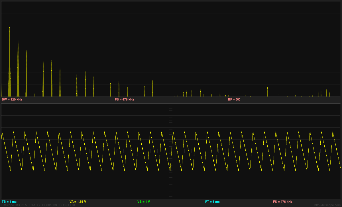
I checked my code by testing with a recording of a triangle wave, and found that Welch’s method with an 80dB Dolph-Chebyshev window did an excellent job of removing the spectral smear that I was getting by just averaging rectangular FFT windows (my first approach). The noise floor for Welch’s method on those measurements was pretty much flat across the entire spectrum (maybe rising at higher frequencies), so the 1/f plot here is not an artifact of the analysis, but a real measurement of the acoustic noise. Using 60dB window resulted in a higher noise floor, but 100dB and larger did not lower the noise floor, so I stuck with 80dB as a good parameter value. It might be useful to use other values if the FFT window width is changed or the noise in the data is different.

I’ve included the source code for the program, so that others can use it. It does require that SciPy be installed, in order to use the scipy.signal package.

#! /usr/bin/env python3

"""Sun Sep  4 21:40:28 PDT 2016 Kevin Karplus

Reads from stdin a white-space separated file 
whose first column is a timestamp (in seconds) and 
whose subsequent columns are floating-point data values.

May contain multiple traces, separated by blank lines.

Outputs a tab-separated file with two columns:
        the frequencies
        the Fourier transform

"""

from __future__ import print_function, division

import argparse
import sys
from math import sqrt
import numpy as np
try:
    from future_builtins import zip
except ImportError:     # either before Python2.6 or one of the Python 3.*
    try:
        from itertools import izip as zip
    except ImportError: # not an early Python, so must be Python 3.*
        pass

import scipy
import scipy.signal

class Trace:
    """One contiguous trace consisting of two 1D numpy arrays of the same length
        times:  timestamps in seconds
        values: arbitrary floats
      and sampling_freq: the sampling frequency in Hz
    """
    def __init__(self,times,values,sampling_freq=None):
        self.times=np.array(times)
        self.values=np.array(values)
        assert self.times.shape==self.values.shape
        if sampling_freq is None and len(times)>1:
            sampling_freq = (len(times)-1)/(times[-1]-times[0])
        self.sampling_freq=sampling_freq
    def __len__(self):
        return len(self.values)

def read_trace(file, column=2, sampling_freq=None, echo_comments_to=None):
    """Generator that yields traces from tab-separated rows of data.
    Each row contains a timestamp in the first column and any number of subsequent
    columns, one of which is selected to be the values for the trace.
    
    New traces are started whenever the timestamp in the first column decreases.
    
    If sampling_freq is None, the sampling_freq for the
    trace is deduced from the timestamps.
    
    Comments and blank lines are echoed to a file-like object,
    echo_comments_to, if it is not None.
    """
    times=[]    # time values (in seconds) from frst column
    values=[]   # values from the specified column
    
    for line in file:
        line=line.strip()
        if line.startswith('#') or len(line)==0:
            if echo_comments_to is not None:
                print(line, file=echo_comments_to)
            continue
        fields=line.split()
        if len(fields)>=column:
            time=float(fields[0])
            if times and time<times[-1]:
                yield Trace(times=times, values=values, sampling_freq=sampling_freq)
                times=[]
                values=[]
            times.append(time)
            values.append(float(fields[column-1]))
    if times:
        yield Trace(times=times, values=values, sampling_freq=sampling_freq)


def posint(opt):
    """returns int(opt) if that is positive,
            otherwise raises an argparse.ArgumentTypeError
    """
    try:
        x = int(opt)
    except:
        x=None
    if x is None or x<=0:
        raise argparse.ArgumentTypeError("{} is not a positive integer".format(opt))
    return x

def parse_options(argv):
    """Parse the options and return what argparse does:
        a structure whose fields are the possible options
    """
    parser = argparse.ArgumentParser( description= __doc__, formatter_class = argparse.ArgumentDefaultsHelpFormatter )
    parser.add_argument("--sampling_freq","-s", type=float,
            default=None,
            help="""Sampling frequency (in Hz). 
            If none specified, then estimate sampling frequency from the timestamps.
            """)
    parser.add_argument("--window", "-w", type=posint,
            default=(1<<16),
            help="""Max window size (in samples) for FFT.
            Longer traces will be split up into windows of this size
            """)
    parser.add_argument("--column" , "-c", type=posint, default=2,
           help="""What column should be Fourier transformed?""")
    parser.add_argument("--welch" , type=float, default=None,
           help="""Use Welch's method to produce averaged spectrum from windows. 
           Value is dB difference between main lobe and sidelobes for Dolph-Chebyshev window. 
           80 seems reasonable with 16-bit data (60 produces a higher noise floor, without noticeably narrowing the spikes).
           Note, sqrt is used to get amplitude spectrum, rather than power spectrum. """)
    options=parser.parse_args(argv[1:])
    return options


def main(argv):
    """parse the command line arguments and do FFTs
    """
    options = parse_options(argv)
    sampling_freq= options.sampling_freq

    # input file may contain separate time traces.
    # Each new trace stats when the time value is less than the previous time.
    
    for trace in read_trace(sys.stdin, column=options.column, 
                        sampling_freq=options.sampling_freq, 
                        echo_comments_to=sys.stdout):
        print("# using sampling frequency {:.6f} Hz for FFT of trace with {} samples".format(trace.sampling_freq,len(trace)))


        fft_len=64      # length of the fft to do
        while fft_len<len(trace) and fft_len<options.window:
            fft_len *= 2
        
        if options.welch is not None:
            welch_f,welch_spectrum = scipy.signal.welch(trace.values, trace.sampling_freq, nperseg=fft_len, scaling="spectrum", window=("chebwin",options.welch))
            print("")       # separate the traces
            for f,w in zip(welch_f,welch_spectrum):
                print("{0:.7f}\t{1:.6f}".format(f, sqrt(w)*(fft_len//2)))
        else:
            for start in range(0,len(trace),fft_len):
                window=trace.values[start:start+fft_len]

                # remove DC component, so that zero-padding makes sense
                # WARNING: This in-place change could introduce errors if
                # overlapping windows are allowed.
                dc = sum(window)/len(window)
                window -= dc

                fft = scipy.fftpack.fft(window, n=fft_len)
                fft[0] += dc

                print("")       # separate the traces
                print("# Window width {} = {:.3f}s".format(fft_len,fft_len/trace.sampling_freq))
                for i,f in enumerate(fft[0:fft_len//2]):
                    print("{0:.7f}\t{1:.6f}".format(i*trace.sampling_freq/fft_len, f))


if __name__ == "__main__" :
    sys.exit(main(sys.argv))

2013 July 10

FFT on ATMega and BitScope

Yesterday, my son was thinking of adding a microphone to the design he is working on, and was considering adding a fast Fourier transform (FFT) to detect pitch.

He spent a few hours after his 10 a.m.–5 p.m. theater class reading about the FFT algorithm. He found an implementation of the FFT for an Arduino, which he tried reading along with the FFT explanations he found on the web.  I’m actually surprised the the Arduino was capable of doing an FFT, given the slowness of the processor.  It is true that the example code only does a 64-sample FFT with a sampling rate of 1kHz, using 8-bit samples and 16-bit integer arithmetic, but it is reported to do it at better than 10 FFTs per second.

I also pointed him to the Discrete Cosine Transform (DCT), which has somewhat smaller boundary artifacts, and can be computed about twice as fast, but he hasn’t had time to read that yet.  Somewhat surprisingly the DCT article in Wikipedia much better written than the general one on Fourier Transforms, which uses awkward notation and a rather dry, formal factoid dump.

I wanted to show him that FFT did not make pitch extraction trivial (at least not in real musical contexts), so I wired up a microphone and amplifier to my BitScope Pocket Analyzer and we turned on some Internet radio (our local public radio station, KUSP).  The complex mass of rapidly shifting peaks in the FFT made it clear that tracking a pitch would not be easy.  (I think that there are some useful pitch-extraction algorithms that are based on FFT, but they are not trivial.) I think I convinced him that he is better off trying to extract loudness than pitch, if he wants a useful control parameter for his device.

Incidentally, he spent some time yesterday looking for cheap electret microphones. There are quite a few on the market, but many of them say “hand solder only” on the datasheets—even some of the ones with just solder pads! There are mics that can be reflow soldered, but finding prices for them in the 100s is difficult—they mostly seem to be quotes from the manufacturers only. One promising one is the SiSonic SPQ2410HR5H-PD, which is only  3.76mm by 2.24mm and uses a ball grid array (it costs 92¢ in 100s, substantially more than 57¢ for the cheapest through-hole mic (though that needs to be hand soldered). CORRECTION 2013 July 10—that’s a MEMS silicon mic, not an electret.

We looked at digital mics that do the A-to-D conversion already, but the only one with a useful output format was the ADMP441, which costs $4.52 in 100s (way too expensive). The cheaper (down to about $1.02) digital mics all use PDM (pulse-density modulation), but to get that into a usable form inside the ATMega, he’d have to low-pass filter it and pass it through the A/D converter. Still, that may not be any more expensive than an analog mic, DC-blocking high-pass filter, and amplifier, though using a separate amplifier would let him design for the proper microphone sensitivity.  He’s going to have to figure out whether the board area and parts cost are worth the extra functionality of the microphone.  If the board area is not a problem, he could design the mic in, but then have the devices only partially populated to save parts costs, if necessary.

We also noticed that we could tell the bandwidth of the radio station we were listening to, because there was a very clear drop in the spectrum at 10kHz.  I tried capturing that this afternoon, but the station we listened to had a talk program rather than a music program, and I never captured a moment when they were using the full bandwidth.  I tried a different Internet music source, and got the following plot, which seemed to indicate a 12kHz bandwidth, but that may have been limited by the music recording they were playing, rather than the codec used for transmission over the internet.

Snapshot of FFT showing a bandwidth of about 12kHz.  The grid for the spectrum is 10dB per division vertically and

Snapshot of FFT showing a bandwidth of about 12kHz. The grid for the spectrum is 10dB per division vertically and 6kHz per division horizontally.

Before we’d played with sound input, we’d looked at sine waves generated by the BitScope, by connecting a wire from the GEN output to the CHA input. I don’t think I was able to explain to him why the windowing function used for removing boundary artifacts in the FFT results in spreading the single-frequency spikes into wider peaks. It was too late at night to go into the theory of transforms and how multiplication in the time domain turns into convolution in the frequency domain, and vice versa. For that matter, he hasn’t even had convolution yet, so some of the fundamentals needed for the explanation were missing.

At one point I thought that the FFT on the Bitscope was a crude rectangular window, but I was informed by the Bitscope people that they use a Kaiser window. I should have been able to tell that they were doing some sort of windowing by seeing the spread of the spikes for sine waves, but I wouldn’t have been able to guess which window. (It may be buried in the documentation somewhere.) Actually, now that I look at the spikes, they seem too wide for a Kaiser window, unless they set the α parameter much too large.  They only need the sidelobes to be about 60dB down, which should be a much narrower main lobe—not the 18-bin width I think I’m seeing. Perhaps there is something else spreading the peaks, not just the Kaiser window.

Sine wave and FFT analysis of it. Note the harmonic distortion (2nd, 3rd, and 4th harmonic)

Sine wave and FFT analysis of it (Click on image for larger, clearer picture). Note the harmonic distortion (2nd, 3rd, and 4th harmonic at about –40dB, –45dB, and —53dB).
Good luck figuring out the settings of the Bitscope from the information they show on the display!  TB is the time per division on the x-axis of the plot, while BW=120kHz is the full width of the spectrum (so 12kHz per division), and the sine wave is at about 3kHz.

It is interesting to look a a sine wave that is an exact submultiple of the sampling frequency:

Here is a 2975Hz sine wave, where each period should be 8 samples long.  Note the appearance of side bands to either side of the main peak.  These artifacts are much smaller if we move to a frequency that does not fit so neatly into the FFT buffer.

Here is a 2975Hz sine wave, where each period should be 8 samples long. Note the appearance of side bands to either side of the main peak. These artifacts are much smaller if we move to a frequency that does not fit so neatly into the FFT buffer.
Note that the time base is different for this screenshot (20ms/division).

We also looked at the spectra of triangle waves and square waves (since the BitScope waveform generator can do those also). Playing with the duty cycle was fun also. I had not been aware that a duty cycle of 1/n on a square wave or triangle wave suppressed the nth, 2nth, 3nth, … harmonics. I had known that a 50% duty cycle square wave or triangle wave suppressed the even harmonics, but I had never thought about other duty cycles.

Triangle wave with 25% duty cycle, showing suppression of the 4th, 8th, 12th, and 16th harmonics.

Triangle wave with 25% duty cycle, showing suppression of the 4th, 8th, 12th, and 16th harmonics.